Durable memory, transient prototypes

Consider a maintenance assistant that needs to decide whether a new incident needs attention. During routine operation, it may compare that incident with one set of past cases. During a planned shutdown, a different set may be relevant. The incident records stay in place while the examples used for the current decision change.

In HDC, a class prototype is a hypervector that summarizes examples from one class for comparison with new queries. Informally, we can think of a prototype as a summary of the essential features of a class. Our experiment keeps the stored examples fixed while building these summaries for each context. We compare rebuilding them with caching them, looking at the predictions they make and the storage and work each approach requires.

In their neuroscience perspective, Barrett and Miller¹ describe situated categories whose prototypes, when present, depend on the goal being served. Barsalou’s earlier work² on ad hoc categories also examines groupings constructed for particular goals, rather than only familiar category structures already established in memory.

These accounts lead us to a practical question for HDC: what should a classifier keep in memory when the goal changes?

A stored summary is one design choice

A concrete precedent for fixed summaries comes from Rahimi and colleagues’ HDC language classifier.³ It accumulates letter-trigram hypervectors into a representation for each language, then compares an unseen text with the stored language representations using cosine similarity.

Our baseline uses the same broad idea of an additive class summary, with synthetic examples instead of text. Each class gets one normalized sum of its training hypervectors. Every query is compared with those two stored prototypes. This baseline is kept deliberately simple; it doesn’t aim to reproduce Rahimi et al.’s language-recognition system.

One stored prototype blends examples from every context, losing the link between each example and its context. Keeping the examples and their context labels lets us select the relevant ones once the context is known.

Bundling gives each class one hypervector to compare with a query. Additively bundling the selected hypervectors reinforces shared elements and partly cancels disagreements. We normalize the real-valued sum to unit length so the prototypes have a consistent scale. Cosine similarity depends only on direction, so this normalization does not change the predictions.

For class $c$, let $M_c$ index its examples and $w_i(L)$ weight example $i$ in context $L$. With $\oplus$ as element-wise addition, the prototype is:

$$\mathbf{h}_{c\mid L} = \frac{\displaystyle\bigoplus_{i\in M_c} w_i(L)\mathbf{h}_i} {\displaystyle\left\|\bigoplus_{i\in M_c} w_i(L)\mathbf{h}_i\right\|_2}.$$

The weights change the contribution of whole examples. In this experiment, a weight is $1$ when an example’s recorded context matches the current context and $0$ otherwise. We construct a prototype for every candidate class, then compare the query with each. The procedure never uses the query’s true class to choose its memories.

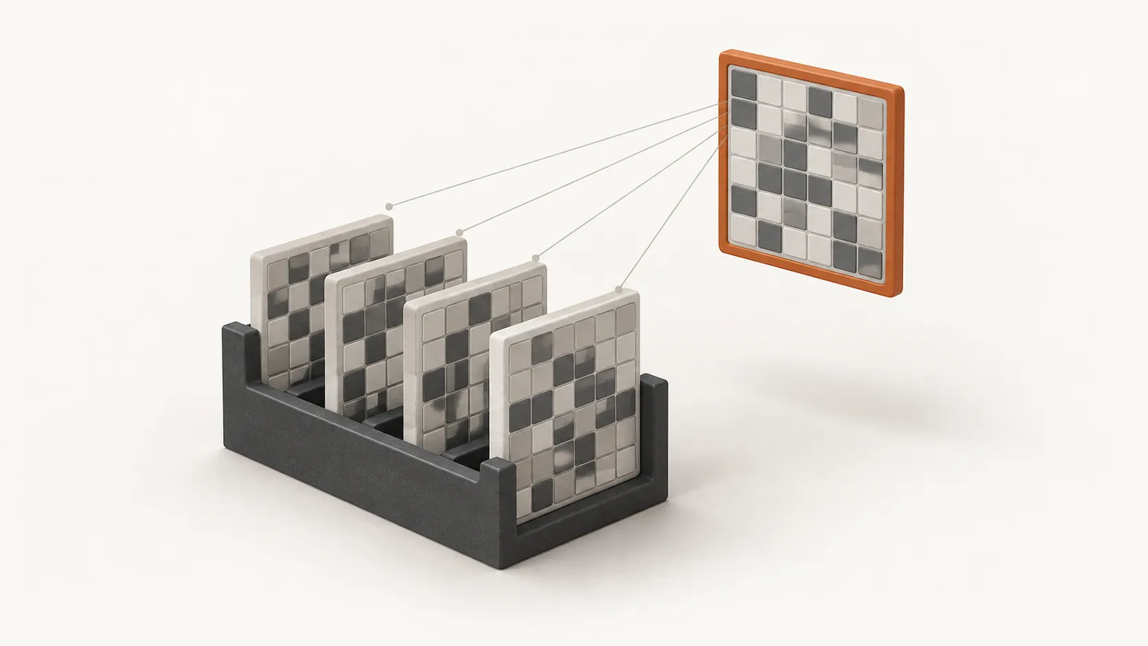
The same stored collection of examples can yield different class prototypes because context determines which examples are bundled.

An experiment with a deliberately changing question

Imagine sorting cards that show one of two patterns. In context A, striped cards belong to Class 0 and spotted cards to Class 1. In context B, the assignments reverse:

Context	Class 0	Class 1
A	Striped	Spotted
B	Spotted	Striped

A striped card looks the same under either rule. If we show it to the classifier twice, the pattern supplies the same evidence both times, while the correct answer changes from Class 0 to Class 1. The classifier needs the active context along with the pattern to make the decision.

Back to the maintenance assistant

Extending the simple example above, our maintenance assistant might receive a report that a machine is offline. During routine operation, that status may call for attention, while during a planned shutdown the assistant might expect it. Both judgments can draw on the same incident history, with the operating mode guiding which past cases are useful.

Why do the labels reverse?

We chose the complete reversal in the card rule to make context matter. If A and B occur equally often, Class 0 gets stripe examples from A and spot examples from B, while Class 1 gets spot examples from A and stripe examples from B. Once we pool those contexts, each class has the same mixture. A classifier using only the card pattern has no dependable way to assign a label.

For the HDC experiment, “striped” and “spotted” are names for two independent random bipolar hypervectors, $\mathbf{h}_u$ and $\mathbf{h}_v$, each with 1,024 components. We make noisy copies of those hypervectors to stand in for imperfect examples of each pattern.

Each class-context combination has 20 training examples, made by independently flipping each component of the corresponding base hypervector with probability 0.20. The test set has 200 new examples per combination, generated with flip probability 0.40. Across ten random seeds, we regenerate the base patterns and examples, giving 8,000 distinct test queries. The context accompanies each query, and no encoder is learned.

What does the classifier keep?

All methods start from the same training examples, so their differences come from what they store and which prototypes they use for a query.

The fixed method pools A and B into one stored prototype for each class. Each prototype contains both stripe and spot examples. The sum carries no record of which example came from which context, so the fixed classifier cannot change its class prototypes when the rule changes.

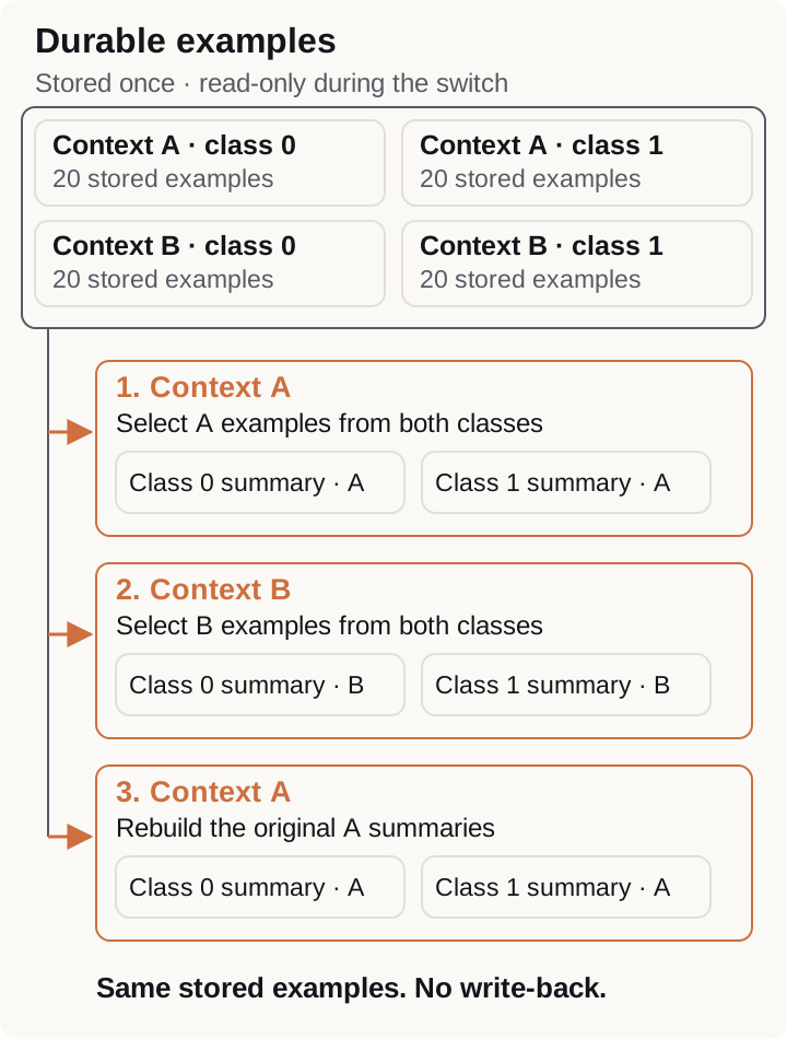
The transient method keeps the examples together with their context labels. When A begins, we bundle its examples into one prototype per class and use that pair for the phase’s queries. When B begins, we build a pair from the B examples. The original examples remain available when A returns.

We can also prepare both pairs ahead of time. The cached method stores four prototypes, one for each class in each context, and uses the pair selected by the query’s context. A wrong-context control deliberately selects the other pair to show what happens when that choice is incorrect.

Once a pair is available, the classifier compares each query with both class prototypes using cosine similarity and predicts the class with the higher score. We use the query’s true class only afterward to measure accuracy. We run A, then B, then A again, reusing the original A queries in the last phase to check whether the same prototypes and predictions return.

The useful result includes the tie

The question is whether each classifier follows the label switch in B and recovers its earlier answers when we return to A. The table shows the percentage of queries it classified correctly in each phase. The last row deliberately selects the wrong context to show what happens when it uses the opposite prototype pair.

Condition	Context A	Context B	Return to A
Fixed	51.1%	49.2%	51.1%
Transient	100.0%	100.0%	100.0%
Cached	100.0%	100.0%	100.0%
Wrong context	0.0%	0.0%	0.0%

The fixed classifier is deterministic: a given query gets the same label in A and B because it is compared with the same two prototypes. The correct label reverses between contexts, so that fixed answer tends to be right in one and wrong in the other. With equally many queries from each context, its 50.1% average is close to the 50.0% expected from a coin flip.

The jump to 100.0% shows what the correct context adds in this constructed test: it selects the prototype pair that follows the current rule. Rebuilding that pair from stored examples and caching it gave identical predictions, so rebuilding brought no accuracy gain here. The test supplied the context. A real maintenance system would have to identify it. The return to A lets us check whether switching contexts disturbed what was stored.

What stayed stable, and what it cost

When A returned, the temporary method rebuilt the same prototypes from the stored examples and gave the repeated A queries the same answers as before. A digital fingerprint of those examples matched before and after every run, confirming that the store stayed unchanged.

We can change the prototypes in use and still recover the earlier decisions from the same stored examples. This test held those examples fixed. To find out whether learning new cases harms earlier memories, we would need to add cases and check what the system remembers afterward.

The accuracy tie leaves a practical question: what does each approach cost to keep and rebuild? The table shows what each method stores and what it needs when the context changes. Each example hypervector uses one byte per component, and each normalized prototype uses eight.

Design	Stored across phases	When context changes
Fixed	Two prototypes (16 KiB)	Keep using the same pair
Cached	Four prototypes (32 KiB)	Select the stored pair
Transient	80 examples (80 KiB)	Build two prototypes (16 KiB)

For these two known contexts, four cached prototypes take 32 KiB and are ready to use. The transient method keeps 80 examples in 80 KiB, then builds a 16 KiB pair from the 40 examples relevant to the current context. It builds that pair once per phase and reuses it for every query. We have yet to measure how much time or energy that work takes.

Both methods got every query right, so keeping the full collection gave no accuracy benefit here. If our maintenance assistant only ever sees routine operation and planned shutdown, two ready-made pairs use less storage and avoid rebuilding. The incident history could matter when a new situation calls for a different choice of past cases, or when an engineer needs to inspect which cases shaped an answer.

Keep the memory and the decision separate

This post covered how predicting a category in HDC doesn’t require us to permanently store one prototype. As developers, the practical choice we make is which information must be kept so the next decision can be constructed faithfully. Sometimes a cached conditional summary is sufficient. Sometimes the system needs richer memories and a temporary view.

Our experiment establishes that separation in a controlled setting, while also exposing its limits: known contexts, synthetic patterns, additional storage, and no learning during the switch. A stronger application test would vary selection weights, introduce context uncertainty, and compare both accuracy and full retrieval costs against caching under the same memory budget.

The natural question that emerges next is how those durable representations were created. A system that learns from a few new examples may already possess a substantial encoder, memory, or set of priors. Our next post examines what the learner already contains before we bring it its first example.

Footnotes

1. Lisa Feldman Barrett and Earl K. Miller, “Categorization is ‘baked’ into the brain” ↗ , Nature Reviews Neuroscience (2026). Open author PDF ↗ , PDF p. 11, discussion of situated prototypes. The paper motivates the question; our read-only memory design and experiment are separate engineering choices. ↩

2. Lawrence W. Barsalou, “Ad hoc categories” ↗ , Memory & Cognition 11 (1983): 211-227. Open institutional copy ↗ . Used for the goal-derived categorization precedent, not as evidence for HDC storage or computation. ↩

3. Abbas Rahimi, Pentti Kanerva, and Jan M. Rabaey, “A Robust and Energy-Efficient Classifier Using Brain-Inspired Hyperdimensional Computing” ↗ , ISLPED (2016). Open author paper ↗ , sections 3.1-3.2. Their fixed language summaries are a computational precedent, not the source of our synthetic results. ↩