When a graph becomes a memory

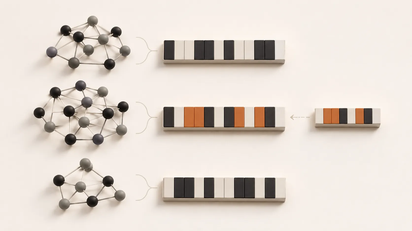
Grouping similar observations can require comparing many of them with one another. Once we’ve found those groups, could we assign new observations by comparing them with just one representative per group? In a recent paper on HDLouvain, researchers find groups using a graph, then represent each group with a binary vector formed by taking a majority vote across its members’ encodings. The question is how much of the group’s structure that vector preserves.

In mass spectrometry, an instrument records patterns of measurements called spectra. Repeated measurements of the same molecule can produce similar patterns, so grouping them can save work during analysis. Finding those groups takes work too: one approach builds a graph connecting similar spectra, then looks for communities within it. Once those communities are known, a new spectrum might be assigned to a group by comparing it with a compact summary of the group’s members.

Beenish Gul and colleagues explore this approach in HDLouvain: High-Throughput Incremental Clustering for Hyperdimensional Data ↗ . They use Louvain community detection to find the initial groups, then bundle each group’s encodings into a binary HDC prototype. Those prototypes form an associative memory that assigns later spectra to groups without repeating the graph analysis.

An interesting question is what survives that step from a graph to a bundled hypervector. A prototype summarizes the patterns shared by a group’s members, but the graph grouped them by their connections to one another. How well does the summary represent the community when new spectral data arrives? We’ll examine the HDLouvain authors’ approach and reported results in the October 22, 2026 arXiv v1 preprint. We haven’t reproduced the measurements.

Let the graph find the groups

The spectra come from tandem mass spectrometry. An instrument fragments a precursor ion and records fragment mass-to-charge ratios and intensities. Repeated measurements of a peptide can produce similar spectra, so clustering them before identification can save redundant work. A useful cluster brings those repetitions together while keeping distinct peptides apart. Split the same peptide across many clusters and much of the redundancy remains; mix different peptides and the cluster becomes a poor basis for identification.

HDLouvain prepares the initial batch of spectra in three steps:¹

Step	What it does
Bucket	Groups spectra by precursor mass to avoid comparing every spectrum with every other spectrum.
Encode	Uses ID-level binding and bundling to combine peak-bin identities and quantized intensities into 2,048-dimensional binary hypervectors.
Connect	Makes those hypervectors the nodes of a weighted nearest-neighbour graph within each bucket.

Each edge needs a weight that measures how similar its two spectra are. HDLouvain compares their binary encodings by the fraction of bits that differ, called the normalized Hamming distance. It converts this distance into a similarity weight:²

$$w_{ij}=1-d_H(\mathbf{h}_i,\mathbf{h}_j).$$

Here, $\mathbf{h}_i$ and $\mathbf{h}_j$ are the two spectra’s encodings, $d_H$ is their normalized Hamming distance, and $w_{ij}$ is the edge weight. Identical encodings get weight 1; more differing bits give a lower weight.

Louvain looks for groups whose internal connection weight exceeds what we’d expect from a degree-preserving null model. In effect, it asks whether these nodes are unusually well connected to each other, given how much connection weight each node has overall. A community can earn a good modularity score without all its members sitting close to one centre. Keep that distinction in mind: it matters when we put the graph away.

The graph is built from an initial batch of spectra, called the bootstrap. Louvain partitions it into communities. Each community then gets one representative binary vector: at each bit position, we take the value that occurs most often among its members’ encodings, choosing zero for ties. This is bitwise majority bundling.

For each later spectrum, its precursor mass selects a bucket. Its encoding is compared with the representatives stored in that bucket. The assignment threshold sets the maximum allowed normalized Hamming distance, or fraction of differing bits. If the closest representative is within that threshold, the spectrum joins its cluster. Otherwise, it starts a new cluster and becomes its representative. Existing representatives stay fixed, however many later spectra join them.¹

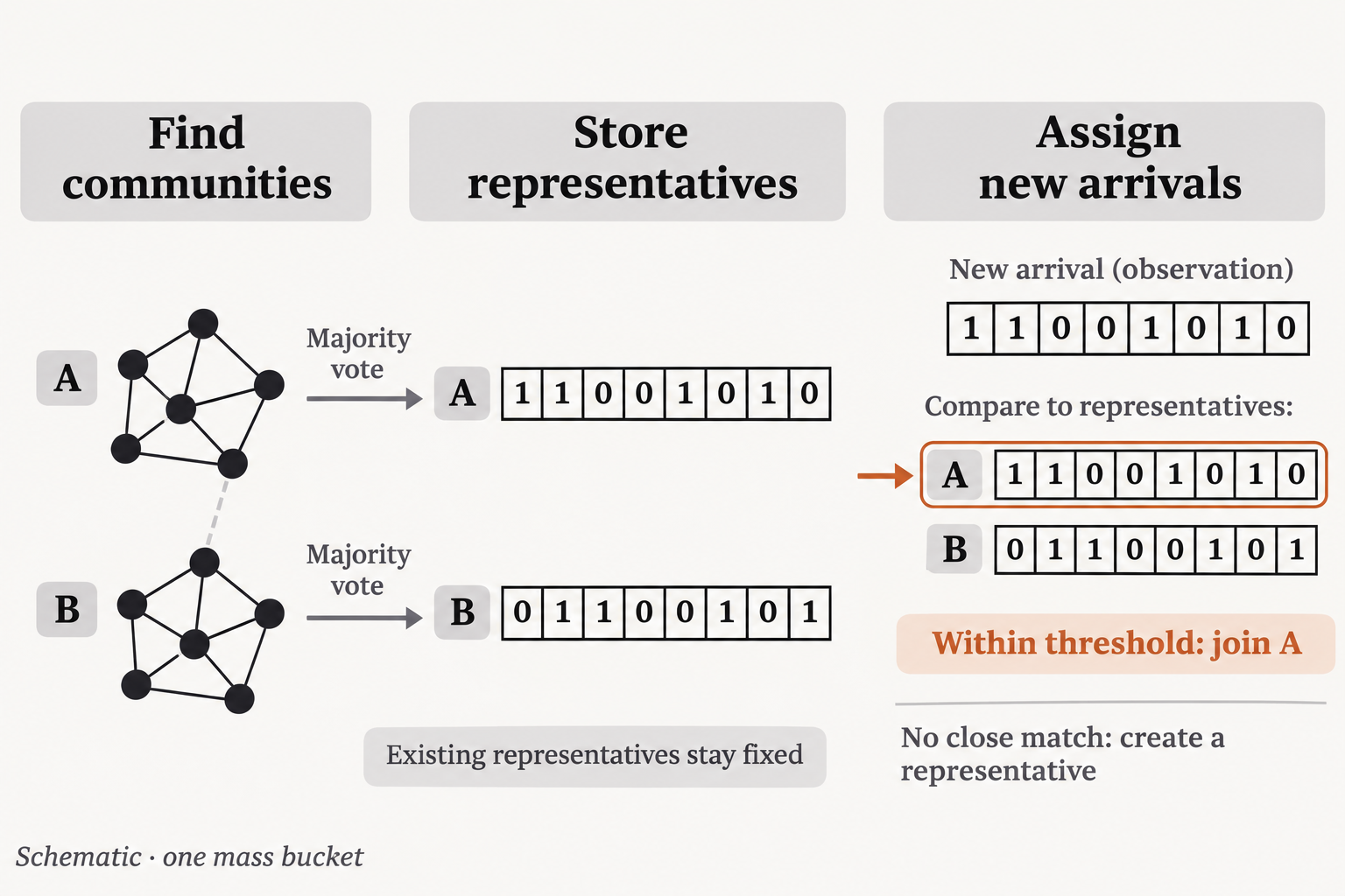
Graph communities become fixed representatives for later spectra. Eight bits shown; the method uses 2,048.

For a community C, we can write its representative using our usual bundling notation:

$$\mathbf{h}_{C}=\bigoplus_{s\in C}\mathbf{h}_{s}.$$

Switching from graph communities to majority representatives changes what it means for our spectrum to belong. During discovery, belonging together meant contributing to a well-connected community. During assignment, it means being close to one majority pattern. The chains, bridges, and dense subgroups in the original graph have disappeared from the decision. We’ve kept a summary of the members, and we’re trusting it to recognize another member when it arrives.

Majority bundling chooses the bit pattern with the smallest total Hamming distance to its inputs: at every coordinate, the majority value incurs the fewest disagreements. A five-bit example shows why that doesn’t promise that every member is nearby.

Member encoding	Bits differing from the majority vector 00000
00000	0 of 5
00000	0 of 5
11111	5 of 5

The majority vector matches two members exactly and disagrees with the third at every bit. This is a toy example of the operation’s limit, not evidence that the measured spectral communities contain such a split.

Our bundling study asked what remains retrievable after superposition. Here the question is whether a discovered community remains recognizable through its bundle. The earlier study used unthresholded bipolar MAP sums, so its measurements don’t transfer directly to binary majority prototypes. Still, the practical concern is familiar: which distinctions survive the summary, and which ones did the next decision need?

Using HDC for spectra has precedents. HyperSpec already combines binary encoding, mass buckets, graphics processing unit (GPU) Hamming calculations, and density-based spatial clustering of applications with noise (DBSCAN) or hierarchical clustering.³ SpecHD takes an HDC spectral pipeline onto a field-programmable gate array (FPGA).⁴ HDLouvain gives the graph a particular job within this line of work: discover the groups that will become an associative memory.

How much faster is it?

The authors compare the time needed to cluster the full dataset with Louvain against the time needed to discover initial groups and assign the remaining spectra through binary representatives. At a 50% bootstrap fraction, Table II reports these mean clustering times over five runs on an RTX 4090 workstation.¹

PRIDE dataset	Spectra	Static Louvain	HDLouvain total	Speedup
PXD001197	992,847	33.5 s	33.0 s	1.0×
PXD001468	1,022,004	37.8 s	34.8 s	1.1×
PXD001511	3,594,140	278.0 s	128.0 s	2.2×
PXD003258	3,700,371	477.7 s	188.1 s	2.5×
PXD000561	21,128,912	10,103.8 s	3,149.0 s	3.2×

The smallest datasets don’t show that much of a benefit. By the time we reach the largest dataset, with over 21 million spectra, HDLouvain shows a 3.21× speedup over the static version. Both methods use the same preprocessing, encoding, bucketing, and graph-construction code. The comparison shows the benefit of running discovery on the bootstrap and assigning the rest through representatives, within this pipeline.

Could clustering be faster if we built the initial graph from a smaller fraction of the spectra and assigned more of them using the stored representatives? In the separate split sweep, a 30% bootstrap reaches 4.5× on PXD003258. The sweep excludes the 21-million-spectrum dataset.¹ We therefore observe two useful results, each tied to its workload and split, rather than a single best-case speedup that applies everywhere.

The binary representation helps make assignment cheap. Storing 32 binary dimensions in one 32-bit machine word lets the processor compare those bits together.⁵ Handling 32 bits at a time doesn’t mean the complete clustering pipeline runs 32 times faster. Encoding, transfers, kernel launches, and bootstrap graph work all remain. The table is the more useful guide to what the authors actually timed; comparisons with other spectral tools or other quantized representations would need further measurements.

Did it keep the right groups?

A useful cluster brings together repeated measurements of the same peptide, a short chain of amino acids. It should keep different peptides apart. The practical question is whether assigning spectra through binary representatives preserves those groups while saving time.

The authors test Louvain on artificial graphs whose groups are known in advance, and it recovers those groups better than the alternatives they tested. This supports the initial group-discovery step. For the real spectra, they use modularity, a score for how strongly connected the nodes are within each group relative to a randomized graph. HDLouvain scores lower than running Louvain on the full dataset, with a reported maximum drop of 8%.¹ That percentage describes a change in graph structure; it isn’t a count of spectra assigned to the wrong peptide.

The diagram shows why peptide identities matter. Both panels contain the same connections, but adding labels reveals that the cluster mixes spectra from two peptides, A and B. To assess the groups, we’d want to check known peptide labels: are different peptides kept apart, and are repeated measurements of the same peptide brought together?

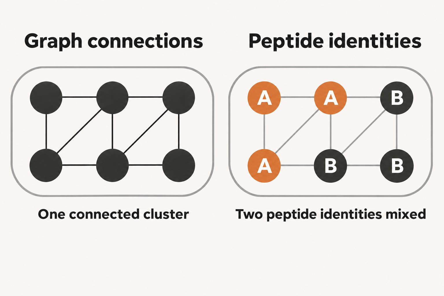
The paper demonstrates faster clustering on its larger datasets. Whether those faster assignments preserve useful peptide groups remains open. A comparison against known peptide identities, using the same data for both methods, would make the practical tradeoff clearer. Some details of the reported comparisons also need clarification.⁶

What happens as new spectra arrive?

Each new spectrum is compared with the representatives in its mass bucket. If it starts a new group, every later spectrum in that bucket must be compared with one more representative.

The table shows how joining an existing group or creating a new one affects later searches:

New spectrum	Assignment	Effect on later searches
Close enough to an existing representative	Joins that group	The number of representatives stays the same.
Too far from every representative	Starts a new group	Every later spectrum in the bucket has one more representative to check.

Existing representatives stay fixed in both cases.¹ That keeps updates cheap, but the search can grow as new groups appear. With 2,048 bits packed into 32-bit words, comparing two vectors takes 64 word comparisons. If a bucket has $R$ representatives, the comparison work for one arrival is therefore:

$$\text{word comparisons per arrival}=64R.$$

For example, 100 representatives require 6,400 word comparisons; 1,000 require 64,000. These are operation counts, not timings: GPU parallelism and other processing costs also affect elapsed time. In the extreme case where every arrival creates a group, each search is longer than the last. The paper does not report this outcome; it is a consequence of the assignment rule.

The initial batch matters too. It determines the groups that later spectra are compared with. During a continuing acquisition, we would need to choose how many spectra, or how much recording time, to use for that first batch. If later measurements differ substantially, the original representatives may become less useful. The authors propose periodic reclustering and cleanup as future work.¹ Rebuilding the groups could help, but its cost would need to be included in the runtime comparison.

What we’d test at HDC Labs

Our reading at HDC Labs suggests a follow-up experiment: test how much of a discovered group’s structure survives in its representative. This is our proposal, not an experiment reported in the paper or one we’ve completed. We’d hold the encoder, mass buckets, initial batch membership, and arrival order fixed, then compare three ways of representing the same groups:

Representative	What the comparison would test
Fixed majority vector, as in HDLouvain	How long the original summary remains useful.
An actual member chosen to minimize total distance to the group, called a medoid	Whether retaining a real member represents the group better than a majority vector.
A representative updated periodically	Whether adapting to later arrivals improves assignments enough to justify the extra work.

A full-data Louvain run would provide a reference. We’d check assignments against known peptide labels and leave unidentified spectra unjudged. Two measurements could help explain mistakes: how far group members lie from their representative, and how much closer each new spectrum is to its best match than its second-best match. A small gap means the assignment is harder to distinguish.

We’d then change the arrival order and introduce peptides absent from the initial batch, tracking grouping accuracy alongside representative count, memory use, and the slowest assignments. Overlapping mass buckets would be a separate test of whether bucket boundaries split measurements that belong together. These are proposed experiments; they require a reproducible implementation and the parameter settings used in the paper.⁷

We’d also compare Louvain with Leiden on the same spectral graphs. Leiden’s original study establishes connectivity guarantees and reports faster execution on its own benchmarks.⁸ The question here is whether its communities produce better representatives and, ultimately, better peptide groups.

Conclusions

HDLouvain offers a concrete way to choose what goes into an HDC bundle: let the graph’s communities determine which observations belong together. The reported runtime gains on larger datasets show why this is worth pursuing. Graph discovery supplies the initial groups, and compact binary representatives make later assignments cheaper.

For us at HDC Labs, the important question is whether those representatives preserve the distinctions that made the groups useful. A majority vector summarizes its members’ bit patterns, but it doesn’t retain their individual connections. Comparing different representatives from the same communities would help establish when that compression is sufficient for assigning new spectra, and when useful information is lost.

The longer-term value depends on how the system handles changing data. New observations may fit existing groups, expose weaknesses in their representatives, or create more groups to search. Measuring assignment quality alongside search and rebuilding costs would show when to keep using the summaries and when to revisit the graph. That is the broader opportunity we see in HDLouvain: using graph structure to build HDC representations whose usefulness can be tested as new data arrives.

Footnotes

1. Beenish Gul, Mahbod Afarin, Farhat Ahmed, Sumukh Pinge, Tsung-Han Lu, Tajana Rosing, and Kevin Skadron. HDLouvain: High-Throughput Incremental Clustering for Hyperdimensional Data ↗ . arXiv:2610.30687v1, October 22, 2026. Method: Algorithm 1 and Sections III-A to III-G. Measurements: Table II and Sections IV-B to IV-D, Figures 3 to 8. Limitations: Sections III-B, III-E, and VI. ↩ ↩² ↩³ ↩⁴ ↩⁵ ↩⁶ ↩⁷

2. HDLouvain, Equation 3 ↗ . Subtracting the normalized distance from 1 gives more similar encodings a higher edge weight. ↩

3. Weihong Xu and colleagues. HyperSpec: Ultrafast Mass Spectra Clustering in Hyperdimensional Space ↗ , Journal of Proteome Research, 2023. The official implementation README ↗ documents the workflow and supported clustering methods; the publisher full text was inaccessible during this review. ↩

4. Sumukh Pinge and colleagues. SpecHD: Hyperdimensional Computing Framework for FPGA-based Mass Spectrometry Clustering ↗ . arXiv v1, November 20, 2023; subsequently published at DATE 2024. See Sections III and IV-E for the architecture and biological quality evaluation. Cross-paper runtimes are not normalized here. ↩

5. HDLouvain, Section III-F ↗ . XOR marks differing bits in each pair of 32-bit words, and a population-count operation totals them; a 2,048-bit vector occupies 64 such words. ↩

6. The comparisons in Sections IV-C and IV-D ↗ need some care. In the synthetic tests, Louvain uses the graph directly, while the other methods use vectors derived from it. Their scores therefore reflect both the input representation and the clustering method. In Figure 5 of the paper, the static Louvain score changes as HDLouvain uses more data to build its initial graph, even though static Louvain is described as using the full dataset throughout. We’d need to know whether its graph or scoring procedure also changed to understand that trend. The caption of the paper’s Figure 8 also compares scores from different initial-data fractions. These issues make the size of the quality tradeoff harder to judge; they don’t show that the clusters are incorrect. ↩

7. In our review, we did not find a release explicitly linked in the paper or locate the evaluated neighbourhood-size and assignment-threshold settings. Reproduction would also need random seeds, graph-scoring code, and timing boundaries. ↩

8. V. A. Traag, L. Waltman, and N. J. van Eck. From Louvain to Leiden: guaranteeing well-connected communities ↗ . arXiv v3, 2019; Scientific Reports 9, 5233. See Sections II to IV for Louvain’s connectivity failure, Leiden’s guarantees, and the authors’ runtime comparisons. ↩