Does HDC fit the physics of light? Reviewing PhotoHDC

Photonics is becoming an infrastructure decision. Light can multiply numbers in a laboratory, but deployed systems also need chips, lasers, memory, interconnects, compilers, and racks. Companies are raising hundreds of millions of dollars to redesign that surrounding infrastructure around optical communication. If we’re willing to change the machine, should we also choose computations that better fit the medium?

In PhotoHDC: An Electro-Photonic Accelerator for Hyperdimensional Computing, the authors argue that Hyperdimensional Computing (HDC) and photonics are unusually well matched.¹ HDC can use low-precision representations and relies heavily on multiplication, accumulation, bundling, and similarity search. Photonic hardware can perform highly parallel linear operations quickly, but conversion, tuning, memory access, noise, and nonlinear functions remain expensive. PhotoHDC attempts to match the algorithm to the hardware.

The paper reports very large energy-delay improvements, so its modeled scope is central to reading the results. We need to ask what the model establishes, which assumptions produce the advantage, and what still needs to be measured before optical HDC becomes a deployment choice.

Why light and HDC might suit each other

Digital computers make multiplication look like one abstract operation. In an electro-photonic accelerator, it is a path through physical components. Electrical values set modulators, light carries signals through waveguides, photodetectors produce currents, and electronic circuits convert, store, route, and normalize the result. The optical multiply-accumulate can be extremely fast even when the machinery around it becomes the limiting cost.

PhotoHDC starts with a traditional HDC encoder that maps an input feature vector $\mathbf{x}\in\mathbb{R}^d$ into a $D$-dimensional hypervector. In the notation used on this site, the encoder is:

$$\mathbf{h}_{x}=B^T\mathbf{x},$$

Each row of $B$ is a base hypervector associated with an input feature. Training bundles encoded examples by class to form class hypervectors. The paper expresses inference, which compares a query with every class hypervector, as another matrix-vector multiplication:

$$\mathbf{s}=C\mathbf{h}_{x}.$$

Each row of $C$ is a class hypervector, and $\mathbf{s}$ contains the similarity scores. The paper uses cosine similarity, with normalization handled outside the displayed matrix product. For this encoder and classifier, the main HDC computation consists of two regular operations that photonic arrays already know how to accelerate.

PhotoHDC also considers record-based encoding. Each feature’s position and quantized value are bound before the results are bundled:

$$\mathbf{h}_{x} = \bigoplus_{i=1}^{d} \left( \mathbf{h}_{\text{position},i} \otimes \mathbf{h}_{\text{level}(x_i)} \right).$$

For the paper’s multi-bit representation, binding becomes element-wise multiplication. After the node hypervectors and neighborhood memories have been prepared, graph encoding follows the same multiply-and-bundle dataflow.

PhotoHDC path	Main operation	What changes in the dataflow
Traditional encoding	Dense projection $B^T\mathbf{x}$	Input tiles can remain stationary while base-hypervector columns stream through the modulators.
Record-based encoding	Position-level binding and bundling	Level values and position values change together, increasing SRAM reads and conversions.
Graph encoding	Node-memory binding and bundling	Reuses the record-based path after graph-specific hypervectors have been precomputed.
Classification	Query-prototype similarity	Encoded queries are compared with class hypervectors in the photonic unit.

The listed dataflows cover a useful subset of HDC workloads, but not all of HDC or Vector Symbolic Architectures (VSA). PhotoHDC doesn’t specify a general path for arbitrary permutation, circular-convolution binding, cleanup memories, sparse block codes, or learned encoders. Its claim is narrower: several common HDC training and classification flows can be arranged around one configurable electro-photonic unit.

What the authors designed

The PhotoHDC core is an array of Mach-Zehnder Modulators (MZMs) and photodetectors. One value controls the modulation of an optical signal; another controls a photodetector’s response. The resulting photocurrent represents their product. Currents from several detectors share a wire, so physical current accumulation performs the addition in a dot product.

Most of the accelerator remains electronic. Static Random Access Memory (SRAM) stores inputs, base hypervectors, level hypervectors, intermediate values, and class hypervectors. Digital-to-Analog Converters (DACs) drive the optical unit. Transimpedance amplifiers and Analog-to-Digital Converters (ADCs) recover results. Switches choose whether currents remain separate for inference or combine across rows for training-time bundling. Digital adders finish partial accumulations.

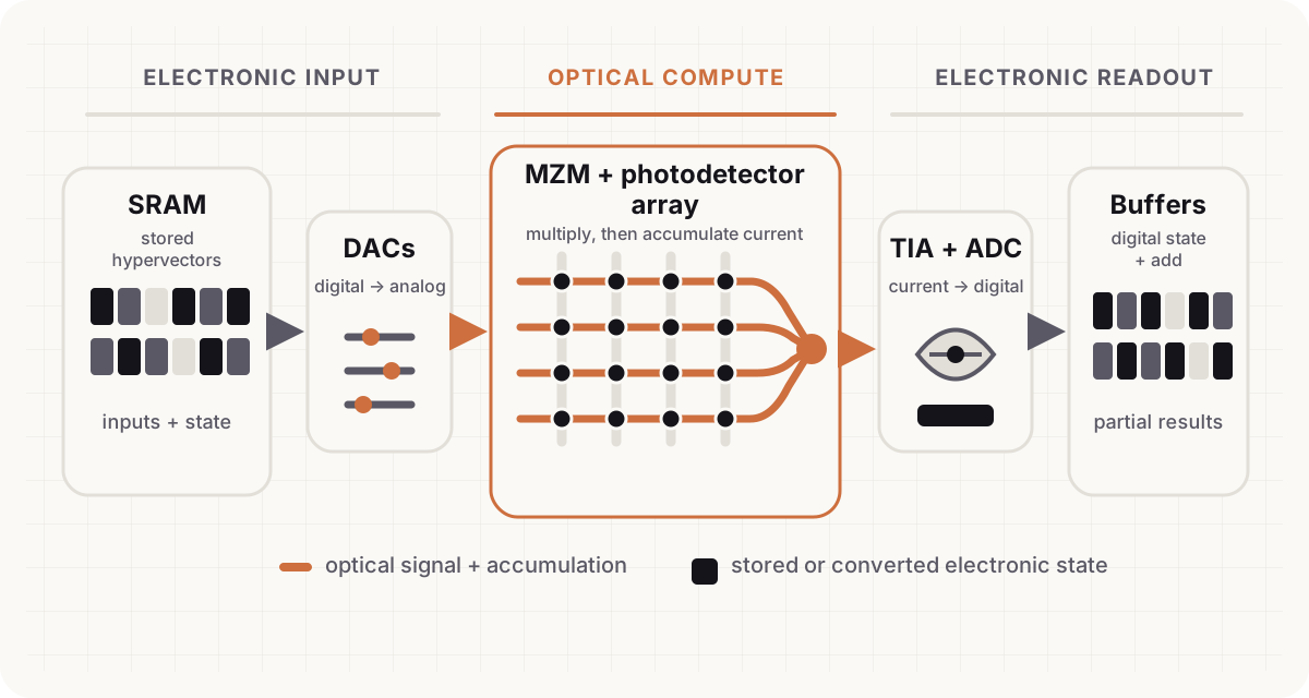
The optical-electronic boundary defines the architecture. PhotoHDC can perform encoding and bundling together during training: samples from one class occupy different photodetector rows, the optical unit produces partial encodings, and the row currents combine before one conversion. For inference, the rows remain separate so each query can be encoded and compared with the class hypervectors.

The design also exposes a difficult conversion trade-off. A 128 × 128 photodetector array would require 16,384 dedicated DACs if every detector were updated independently. PhotoHDC instead lets one DAC program several detectors in sequence, reducing area but adding tile-loading delay. Traditional encoding can hide much of the delay by reusing an input tile for many operations. Record-based and graph encoding can’t hide it as easily because their detector values change every cycle.

The results map the bottlenecks

The journal version evaluates five conventional datasets (ISOLET, UCIHAR, FACE, PAMAP, and PECAN) and three graph datasets (DD, ENZYMES, and PROTEINS). Every experiment uses four-bit values and $D=4{,}096$. The design search selects configurations under a 20 W power budget and a $500\,\text{mm}^2$ area budget.

The authors report that PhotoHDC achieves one to four orders of magnitude lower Energy-Delay Product (EDP) than three electro-photonic DNN accelerators mapped to traditional HDC encoding, while improving modeled area efficiency by roughly one order of magnitude on average. Against a Resistive RAM (ReRAM) compute-in-memory baseline produced with DNN+NeuroSim, the paper reports three orders of magnitude lower EDP for training and inference.¹

Reported comparison	Workload and conditions	What the result supports
ADEPT, DEAP-CNN, and Albireo	Traditional HDC encoding; competitor converter power scaled to four bits	A workload-specific photonic dataflow can outperform photonic designs optimized for different neural workloads in this model.
ReRAM compute-in-memory	Traditional encoding modeled as fully connected layers in DNN+NeuroSim	Fast multi-bit updates and optical accumulation can win on EDP against this selected ReRAM configuration.
Record-based and graph paths	PhotoHDC design-space exploration only	The architecture can express the operations, but it does not provide the same external accelerator comparison.

The component breakdowns are more informative than the headline orders of magnitude. For traditional encoding, MZM tuning accounts for more than half of modeled power, while SRAM movement contributes about 23%. For record-based encoding, repeated tile updates make SRAM the dominant power cost; graph encoding follows the same trend. In the ISOLET traditional-encoding configuration, DACs occupy more than 70% of modeled chip area.

Once the optical dot product stops being the bottleneck, programming, memory, and conversion take its place. Traditional encoding benefits because it reuses stationary data. Record-based encoding is less naturally aligned with the array because its values change together. Whether HDC fits photonics therefore depends on the HDC algebra, representation, update schedule, and memory path.

How far the evidence goes

The final PhotoHDC journal article² narrows the preprint’s headline EDP claims: two to five orders of magnitude becomes one to four against photonic-DNN designs, while four orders becomes three against compute-in-memory. The public record doesn’t explain the revision, so this review reports those values without attributing a cause.

The paper also acknowledges that its datasets are small and simple. It omits accuracy comparisons with conventional DNNs, relying on prior HDC studies, and fixes arithmetic at four bits. That choice reduces modeled converter and laser costs, but the paper gives no end-to-end accuracy-efficiency curve for PhotoHDC.

Missing evidence	Why it matters
Fabricated end-to-end accelerator	System-level optical loss, crosstalk, drift, calibration, packaging, and thermal behavior can interact in ways component estimates do not capture.
Accuracy and similarity degradation	HDC’s general tolerance to noise does not guarantee that every task retains its class ordering, binding inverse, or cleanup margin after a coherent analog distortion.
Shared implementations across hardware	Part of PhotoHDC’s advantage comes from specialization, while the DNN comparators are executing a workload they were not designed for.
Broader HDC operations	The evaluated dataflows do not establish support for the full range of HDC/VSA representations and algebras.
Public result artifacts	We did not locate official code, simulator configuration, or per-experiment result files with which to reproduce the published tables.

The compute-in-memory comparison needs similar care. It uses one ReRAM model, maps traditional HDC operations as fully connected layers, and retains many DNN+NeuroSim defaults. Record-based encoding is excluded because that simulator cannot express it through the same mapping.

The baseline experiment is legitimate, but it doesn’t establish that photonics dominates every existing or future compute-in-memory implementation of HDC. Prior work has already demonstrated physical in-memory HDC systems and hardware-aware retraining , so photonics and memory remain competing design choices rather than a settled hierarchy.

OLIX as a commercial counterpoint

OLIX provides a commercial counterpoint to PhotoHDC. On August 3, 2026, the company announced a $312 million Series B at a reported $3.3 billion valuation. OLIX says the financing will support its path to first DX-1 customer racks in the second half of 2027.³

The financing shows that investors, semiconductor partners, and an engineering organization are willing to fund chips, lasers, compilers, supply chains, and rack-scale optical systems. It provides no evidence that PhotoHDC’s modeled EDP will appear in silicon.

Publicly described PhotoHDC strategy	Publicly described OLIX strategy
Use photonics for HDC multiplication, accumulation, bundling, and similarity.	Use a “slow and wide” optical interconnect to move data directly between chips.
Choose HDC partly because low-precision linear operations suit the medium.	Keep models in fast on-chip SRAM and preserve compatibility with models as they exist today.
Specialize one accelerator around selected HDC dataflows.	Unroll model stages across specialized chips while retaining a flexible compute fabric.
Evaluate training and inference as an architecture study.	Initially target frontier-model decode at rack scale.

OLIX’s manifesto states that a successful alternative shouldn’t require quantization-aware training or post-training quantization of existing models. Its public architecture places the optical emphasis on interconnect and data movement around SRAM-rich compute.⁴ OLIX hasn’t publicly described an HDC accelerator or a PhotoHDC-like photonic multiply-accumulate fabric.

OLIX is a counterpoint rather than a direct application of PhotoHDC. Both projects begin with the cost of moving data and the need for system-level co-design, then take different routes:

1. Preserve the model and redesign movement by keeping contemporary neural inference intact while replacing expensive electrical communication with optical links.
2. Choose a model that fits optical computation. HDC’s precision and operation mix may reduce the conversions and nonlinear support that burden photonic neural accelerators.

The two strategies can coexist. A future rack could use optical interconnect between electronic accelerators, photonic compute for selected kernels, and HDC for associative or symbolic stages. Funding for the first strategy can’t serve as experimental confirmation of the second.

Optical HDC beyond PhotoHDC

PhotoHDC first appeared as a preprint in 2023. Later work now spans modeled accelerators, optical representations, application-specific systems, enabling components, and physics-native proposals.

Evidence level	Example	What it adds
Modeled HDC accelerator	OpticalHDC	Configurable microring cores for HDC encoding and classification, with modeled speedups over ASIC and GPU baselines.5
Optical HDC representation	Speckle-based soft sensing	Experimental optical mapping of sensor inputs into more than 250,000 dimensions for touch and tactile recognition.6
Application-specific architecture	Opto-Aligner	A near-sensor silicon-photonic HDC path for genomic pre-alignment, offering a candidate workload where very high throughput matters.7
Hybrid neural-symbolic system	Neuro-Photonix	Photonic neural processing combined with HDC hypervector generation rather than treating HDC as a DNN replacement.8
Enabling memory primitive	X-pSRAM	Photonic SRAM with embedded XOR, a potentially useful primitive for binary binding rather than a complete HDC system.9
Physics-native HDC/VSA	Wave-geometric duality	Bundling, permutation, binding, and similarity mapped to wave superposition, phase evolution, nonlinear mixing, and differential readout.10

The speckle-based sensing work stands apart because it uses the physical optical response itself as a high-dimensional mapping and demonstrates adaptive recognition. Opto-Aligner addresses a different question: genome filtering is closer to the kind of sustained, data-intensive HDC workload that might justify specialized photonics.

The wave-geometric proposal takes a different step. PhotoHDC maps selected HDC operations onto a familiar multiply-accumulate architecture. Wave-geometric HDC asks whether the algebra can emerge from wave physics itself: superposition for bundling, phase shifts for permutation, nonlinear spectral mixing for binding, and power readout for similarity. Its results remain simulation-heavy and expose difficult coherence and readout constraints, but the proposal expands what “hardware-algorithm fit” might eventually mean.

The HDC Labs perspective

In our review of hardware-aware HDC , we asked whether a learnable encoder could shape hypervector geometry around a modeled device response. PhotoHDC reverses the question: instead of training the representation to tolerate whichever device we selected, can we choose hardware whose natural operations already preserve what the representation needs?

The answer depends on which property must survive. A prototype classifier needs the correct class score to remain first. Binding and unbinding need the desired term to remain separable from cross-term noise. Graph memorization may require neighborhood structure to survive composition. Evaluating an optical implementation therefore requires the similarity rankings, decision margins, inverse relations, and cleanup behavior left after the complete physical path, alongside operations per second and aggregate arithmetic error.

A fuller co-design target is as follows:

$$\begin{aligned} \text{useful optical HDC} ={}& \text{representation} \\ &+ \text{movement} \\ &+ \text{conversion} \\ &+ \text{composition} \\ &+ \text{readout} \end{aligned}$$

Optimizing only the photonic multiply-accumulate can move the bottleneck to DACs, SRAM, tuning, or calibration. PhotoHDC’s own breakdowns show this migration. Optimizing only the HDC algorithm can produce a lightweight digital workload that is too small to amortize an optical system. The useful region is where a high-rate application needs HDC’s associative or compositional behavior often enough to keep the optical path busy.

The paper suggests graph processing, genomics, and datacenter HDC as possibilities. We’d put the workload question at the center of the next study. A photonic HDC accelerator justifies its cost only when the complete application creates enough repeated, structured work to justify lasers, converters, memory, packaging, cooling, compilation, and calibration.

Experiments we would run next

A future study should connect the clean architectural model to a measured task.

1. Calibrate the optical model against fabricated MZMs, photodetectors, converters, waveguides, and packaging across temperature, process variation, and drift.
2. Measure HDC geometry by reporting class margins, pairwise rank correlation, unrelated-item similarity, bundle signal-to-noise, and unbinding error alongside application accuracy.
3. Sweep dimension, precision, sparsity, encoder family, binding algebra, prototype count, and update frequency instead of fixing $D=4{,}096$ and four bits.
4. Use one implementation to compare CPU, GPU, digital ASIC, compute-in-memory, OpticalHDC, and PhotoHDC with matched datasets, preprocessing, precision, accuracy, and system boundaries.
5. Choose a scale-appropriate workload such as sustained genome filtering, high-rate associative retrieval, graph memorization, or a hybrid neural-symbolic serving stage rather than relying only on small classification datasets.
6. Account for the rack by including laser efficiency, conversion, SRAM, tuning, cooling, optical and electrical networking, compiler scheduling, utilization, and host coordination.
7. Publish the simulator configuration, component models, mapping code, seeds, per-run results, and a path from application accuracy to PPA estimates.

We’d compare two optical strategies on the same hybrid workload. The first would keep a conventional neural model and use photonics only for interconnect or dense tensor operations. The second would hand an associative, retrieval, or reasoning stage to HDC on a PhotoHDC-like core. The experiment would turn the OLIX-PhotoHDC contrast from an editorial framing into a measurable partitioning decision.

Where PhotoHDC leaves us

The PhotoHDC research paper doesn’t establish that HDC will be the winning workload for photonic computing. Its accelerator is modeled rather than fabricated, its datasets are deliberately modest, its accuracy isn’t reported, and its largest comparisons depend on mapping HDC to systems designed for other workloads.

PhotoHDC shifts the question away from how efficiently emerging hardware imitates a generic tensor processor and toward which computational model suits the hardware. HDC has a different mix of operations, precision, state, and robustness, and PhotoHDC shows how those differences can reshape a photonic dataflow. Its power and area breakdowns also show that the surrounding electronic system remains part of the computation.

OLIX’s financing makes the infrastructure problem commercially immediate, but it doesn’t settle the research question. Publicly, OLIX is betting on optical movement around SRAM and existing models. PhotoHDC asks whether some stages should instead use a computational model chosen for light. New evidence now needs to show where that choice wins after accuracy, fabrication, memory traffic, conversion, and system utilization are all counted.

Footnotes

1. Farbin Fayza et al., “PhotoHDC: An Electro-Photonic Accelerator for Hyperdimensional Computing” ↗ , ACM Journal on Emerging Technologies in Computing Systems 22, no. 3 (2026), article 16. ↩ ↩²

2. Farbin Fayza et al., “Towards Efficient Hyperdimensional Computing Using Photonics” ↗ , arXiv:2311.17801v2 (2024). ↩

3. OLIX, “OLIX raises $312m at a$3.3bn valuation and appoints Professor Nick McKeown to its board” ↗ , August 3, 2026. The valuation, product-performance statements, and H2 2027 delivery target are company claims. ↩

4. OLIX, “Compute Manifesto: The Inference Era” ↗ (2026). This is OLIX’s account of its architecture and market thesis, not independent product validation. ↩

5. Jiaqi Liu and Yiwen Ma, “OpticalHDC: Ultra-fast Photonic Hyperdimensional Computing Accelerator” ↗ , Proceedings of ASP-DAC (2025): 748–753. Only the publisher/program abstract and metadata were openly accessible during this review. ↩

6. Kei Kitagawa et al., “Optical Hyperdimensional Soft Sensing: Speckle-Based Touch Interface and Tactile Sensor” ↗ (2024 preprint). ↩

7. Deniz Najafi et al., “Opto-Aligner: Optical Near-Sensor Architecture for Accelerating DNA Pre-Alignment Filtering” ↗ , IEEE Journal on Emerging and Selected Topics in Circuits and Systems 16, no. 1 (2026): 124–136. ↩

8. Deniz Najafi et al., “Neuro-Photonix: Enabling Near-Sensor Neuro-Symbolic AI Computing on Silicon Photonics Substrate” ↗ (2024 preprint). ↩

9. Md Abdullah-Al Kaiser et al., “X-pSRAM: A Photonic SRAM with Embedded XOR Logic for Ultra-Fast In-Memory Computing” ↗ (2025 preprint). ↩

10. Tyler L. Poore, “A Wave–Geometric Duality for Hyperdimensional Computing” ↗ (2026 preprint). ↩

11. Christos Pappas et al., “A 262 TOPS Hyperdimensional Photonic AI Accelerator Powered by a Si3N4 Microcomb Laser” ↗ (2025 preprint). ↩

12. S. Kovaios et al., “On-Chip 1 TOPS Hyperdimensional Photonic Tensor Core Using a WDM Silicon Photonic Coherent Crossbar” ↗ (2026 preprint). The paper reports 0.96 TOPS for the demonstrated core. ↩