The (not so surprising) similarities between HDC algebras

Our earlier post on the brief history of vector symbolic architectures traced the development of HDC/VSA and their shared goal of representing and manipulating structured information using high-dimensional vectors. In this post, we’ll look at three influential HDC architectures and the similarities between them.

If we had to condense more than 30 years of HDC research into a compact summary, the work of Tony Plate, Pentti Kanerva, and Ross Gayler would provide a concrete spine, as their work (through a spate of influential papers) laid the foundation for three prominent HDC architectures.

The table below highlights the hypervector space used by each architecture they introduced. In this post, we’ll cover only these three architectures, but bear in mind that many other HDC/VSA approaches exist, and they can be understood as variations on the same theme.

Researcher	Architecture	Hypervector space
Tony Plate1	Holographic Reduced Representations (HRR)	Real-valued
Pentti Kanerva2	Binary Spatter Codes (BSC)	Binary
Ross Gayler3	Multiply-Add-Permute (MAP)	Bipolar

In this post, we’ll see how all three are conceptually similar under the hood despite using fundamentally different numerical representations in their algebras.

A simple computation

Consider an object in the real world that has three attributes:

COLOR = red
SHAPE = circle
SIZE = small

Encoding such a record requires us to associate (bind) each role with its value and then combine (bundle) the three associations into one hypervector. Afterward, we should be able to use the COLOR role hypervector to unbind the record and produce a hypervector similar to red.

The abstract computation can be expressed as follows:

$$\mathbf{h}_{\text{record}} = \operatorname{bind}(\mathbf{h}_{\text{color}},\mathbf{h}_{\text{red}}) \oplus \operatorname{bind}(\mathbf{h}_{\text{shape}},\mathbf{h}_{\text{circle}}) \oplus \operatorname{bind}(\mathbf{h}_{\text{size}},\mathbf{h}_{\text{small}})$$

A generic mathematical notation is used here for binding and bundling. But the important point is that the same abstract computation is carried out in each algebra, even if the underlying hypervector space and binding operation may be different.

The operators (binding, bundling, and unbinding) describe what the representation needs to do, while the algebra describes the underlying numerical machinery and how those operators compose.

Comparing the different algebras

For the algebras to work, the object’s meaning must remain invariant across representations. COLOR = red should represent the same fact whether its hypervectors contain bits, bipolar values ($\pm1$), or floats. What differs is how each algebra forms the associations, combines them, and reverses the operations later.

In the sections below, we’ll follow the same set of operations across the three algebras, asking the same questions each time:

• What happens to the components during binding?
• Does unbinding reverse the operation?
• What remains once several associations have been bundled together?

Unbinding uses a role hypervector to recover its associated value. Its output is another hypervector, not the symbolic label red. Unbinding COLOR reverses the COLOR = red binding, but it doesn’t remove the bundled SHAPE = circle and SIZE = small associations. The resulting hypervector therefore differs from red coordinate by coordinate while remaining similar to it overall.

A nearest-neighbor search can map the recovered hypervector back to a symbolic value by finding the stored value hypervector with the highest similarity.

BSC

Let’s begin by understanding Kanerva’s Binary Spatter Codes. BSC uses binary hypervectors and XOR (exclusive OR) for binding. The hypervectors are typically thousands of dimensions long, but in the sections below, we illustrate the operations with a small hypervector containing just six elements.

The COLOR role and the value red are represented as follows:

$$\begin{aligned} \mathbf{h}_{\text{color}} &= [0, 1, 1, 0, 1, 0] \\ \mathbf{h}_{\text{red}} &= [1, 0, 1, 1, 0, 0] \end{aligned}$$

BSC: Binding with XOR

XOR⁴ works through the two hypervectors one position at a time, asking a simple question at every coordinate: are the bits the same or different? Matching bits produce $0$, while non-matching bits produce $1$. Each output bit depends only on the input bits at the same position in the two hypervectors:

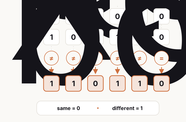
The bound hypervector is dissimilar to both its constituents COLOR and red, but the change doesn’t erase the relationship between them: using COLOR as a cue returns red exactly because XOR is self-inverse. Kanerva therefore used the same $\otimes$ operator⁵ for unbinding:

$$(\mathbf{h}_{\text{color}} \otimes \mathbf{h}_{\text{red}}) \otimes \mathbf{h}_{\text{color}} = \mathbf{h}_{\text{red}}$$

Our record contains two other associations, SHAPE = circle and SIZE = small. BSC binds those pairs in exactly the same way.

BSC: Bundling with majority voting

Once we have the three bound results, we can bundle them. BSC does this with an element-wise majority vote across the bound hypervectors⁶ . If two or more inputs contain a $1$, the bundle receives a $1$ at that position; otherwise, it receives a $0$. Repeating the vote across every coordinate produces one hypervector with the same width as the inputs. Unlike binding, the bundled result remains similar to its constituent hypervectors.

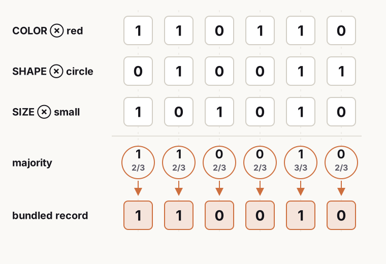
XOR exactly unbinds an isolated COLOR = red pair. After majority voting, however, some bits from that pair have been replaced by the vote across all three associations. XORing the bundle with COLOR therefore returns a hypervector similar to red, not an exact copy.

BSC gives us our first concrete implementation: XOR handles binding and unbinding, while majority voting handles bundling.

MAP

In Gayler’s Multiply-Add-Permute (MAP), the hypervectors are bipolar, meaning every component is either $+1$ or $-1$. As a result, it replaces BSC’s XOR and majority vote with element-wise multiplication and addition. In fact, MAP can be understood as a simple re-encoding of BSC’s bits into bipolar values via the following correspondence:

$$0 \leftrightarrow +1, \qquad 1 \leftrightarrow -1$$

MAP: Binding is element-wise multiplication

Multiplication gives MAP its own means to check for agreement between components: equal signs produce $+1$, while different signs produce $-1$. Each output coordinate corresponds to the result produced by XOR in BSC, even though MAP obtains it through multiplication over signs.

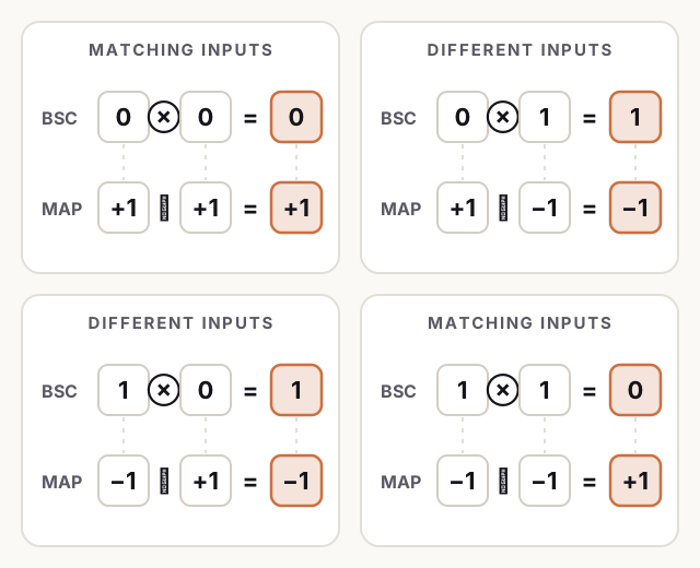
For our COLOR = red example, the MAP hypervectors are:

$$\begin{aligned} \mathbf{h}_{\text{color}} &= [+1, -1, -1, +1, -1, +1] \\ \mathbf{h}_{\text{red}} &= [-1, +1, -1, -1, +1, +1] \end{aligned}$$

MAP binds them by multiplying corresponding components element-wise:

$$\mathbf{h}_{\text{color}} \odot \mathbf{h}_{\text{red}} = [-1, -1, +1, -1, -1, +1]$$

MAP’s bipolar hypervectors make binding exactly self-inverse, just like BSC’s XOR. Unbinding the COLOR role from the bound result therefore recovers red exactly:

$$(\mathbf{h}_{\text{color}} \odot \mathbf{h}_{\text{red}}) \odot \mathbf{h}_{\text{color}} = \mathbf{h}_{\text{red}}$$

MAP: Bundling is addition

Bundling in MAP is simple: it adds corresponding components. Here’s what bundling preserves for the first three coordinates of three bound hypervectors:

$$\begin{aligned} \mathbf{h}_1 &= [+1, +1, -1] \\ \mathbf{h}_2 &= [+1, +1, +1] \\ \mathbf{h}_3 &= [+1, -1, -1] \\ \mathbf{h}_{\text{bundle}} &= \mathbf{h}_1 + \mathbf{h}_2 + \mathbf{h}_3 \\ &= [+3, +1, -1] \end{aligned}$$

Unlike BSC, which keeps only the winning bit, MAP retains the vote margin at each coordinate. Agreement reinforces the magnitude, while disagreement cancels toward zero: $+3$ records three votes for $+1$, whereas $+1$ records a two-to-one split. Taking the sign discards this margin and keeps only the majority result.

HRR

MAP is conceptually close to BSC, while HRR looks different on the surface: its hypervectors contain real values, and it uses circular convolution ($\circledast$) to perform binding. To see HRR’s similarity to MAP, we first need to understand why Plate chose circular convolution.

HRR: Circular convolution compresses pairwise interactions

Our earlier history post on VSA⁷ introduced HRR as Plate’s answer to the dimensionality problem created by Smolensky’s Tensor Product Representations. Smolensky bound a $D$-dimensional role to a $D$-dimensional filler using their outer product:

$$\mathbf{T} = \mathbf{h}_{a}\mathbf{h}_{b}^{\mathsf{T}} \in \mathbb{R}^{D \times D}$$

The outer product retains every pairwise interaction between the inputs, but the result contains $D^2$ components and no longer lives in the same space as either input. Binding the result again would introduce another tensor dimension.

Plate’s goal was to keep the bound result inside the original $D$-dimensional space. Circular convolution does this by assigning the $D^2$ pairwise products to $D$ wrapped diagonals and summing each group into one output coordinate:

$$(\mathbf{h}_{a} \circledast \mathbf{h}_{b})_k = \sum_{i=0}^{D-1} h_{a,i}\,h_{b,(k-i)\bmod D}$$

With the same six-dimensional setup used throughout this post, the two inputs are:

$$\begin{aligned} \mathbf{h}_{a} &= [h_{a,0}, h_{a,1}, h_{a,2}, h_{a,3}, h_{a,4}, h_{a,5}] \\ \mathbf{h}_{b} &= [h_{b,0}, h_{b,1}, h_{b,2}, h_{b,3}, h_{b,4}, h_{b,5}] \end{aligned}$$

Their outer product contains $6^2 = 36$ products. Circular convolution distributes those products across six output coordinates, so the first output coordinate sums this wrapped group of six:

$$\begin{aligned} (\mathbf{h}_{a} \circledast \mathbf{h}_{b})_0 &= h_{a,0}h_{b,0} + h_{a,1}h_{b,5} + h_{a,2}h_{b,4} \\ &\quad+ h_{a,3}h_{b,3} + h_{a,4}h_{b,2} + h_{a,5}h_{b,1} \end{aligned}$$

Every pair whose indices wrap back to position $0$ contributes to that output coordinate. The other five coordinates collect the other wrapped groups, accounting for all 36 pairwise products exactly once. The compression comes from summing each group, so the individual products no longer occupy separate coordinates.

MAP writes one product into each output coordinate. HRR mixes six products into each coordinate, yet still returns a six-dimensional hypervector that can participate in another binding operation. More generally, two $D$-dimensional inputs produce one $D$-dimensional bound representation.

HRR in Fourier space starts to look like MAP

Circular convolution in HRR might be compact from a mathematical perspective, but from an implementation perspective, it’s more complex than MAP or BSC. However, there’s a nice trick that’s useful in practice: remapping HRR into Fourier space makes it a lot easier (and faster) to compute.

A Fourier transform re-expresses the same information in a different coordinate system called the frequency domain. The transformation is invertible, so we can move into Fourier coordinates and back again.

Let $\mathcal{F}$ denote the discrete Fourier transform. Then, the circular convolution of two hypervectors $\mathbf{h}_{a}$ and $\mathbf{h}_{b}$ can be expressed in Fourier space as:

$$\mathcal{F} \left( \mathbf{h}_{a} \circledast \mathbf{h}_{b} \right) = \mathcal{F}(\mathbf{h}_{a}) \odot \mathcal{F}(\mathbf{h}_{b})$$

This makes things much simpler: the same coordinate mixing we saw above becomes element-wise multiplication after the change of coordinates. To return the bound hypervector to the original space, we apply the inverse Fourier transform:

$$\mathbf{h}_{a} \circledast \mathbf{h}_{b} = \mathcal{F}^{-1} \left( \mathcal{F}(\mathbf{h}_{a}) \odot \mathcal{F}(\mathbf{h}_{b}) \right)$$

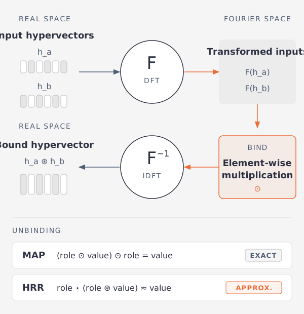
Unlike MAP (where binding is self-inverse), HRR can’t use the same operation because its Fourier components aren’t generally self-inverse. It instead uses circular correlation ($\star$) to unbind the record:

$$\mathbf{h}_{\text{color}} \star \left( \mathbf{h}_{\text{color}} \circledast \mathbf{h}_{\text{red}} \right) \approx \mathbf{h}_{\text{red}}$$

In Fourier space, HRR binds a role and value by multiplying their corresponding components. Reversing that operation exactly would require dividing by the role. Circular correlation instead multiplies by the role’s complex conjugate, which cancels the role’s phase, but it only cancels the magnitude when every component has magnitude $1$. As a result, HRR recovers a value that is only approximately equal to the original.

The algebra is just a design choice

BSC, MAP, and HRR use different vector spaces and express the operations of HDC differently, yet they arrive at the same larger computational shape.

When we place these architectures side by side, both their differences and similarities become much easier to see.

Property	BSC	MAP	HRR
Hypervector space	Binary	Bipolar	Real-valued
Binding	XOR	Element-wise multiplication	Circular convolution
Unbinding	XOR	Multiplication	Circular correlation
Reversibility of binding	Exact	Exact	Approximate
Bundling	Majority vote	Addition	Addition
Dimensionality of bound result space	$D$	$D$	$D$

The hypervectors for each algebra live in different geometrical spaces, and their recovery properties might differ. But there’s a larger common structure underneath. All three algebras give us a way to associate, compose, and recover information without leaving the original hypervector space.

MAP’s bipolar algebra is appealing when we want simple, exactly self-inverse binding. HRR becomes particularly interesting when the algebra itself needs to represent transformations: with unitary vectors, repeated and even fractional binding can encode positions, displacements, or other continuous quantities while remaining exactly reversible.

In the end, the choice of algebra is a design decision that depends on the application and the properties we want to preserve. But the underlying HDC computation shape is largely the same.

Footnotes

1. Tony Plate, “Holographic Reduced Representations” ↗ (1995). Plate uses circular convolution to bind real-valued hypervectors while keeping the result in the same fixed-dimensional space. ↩

2. Pentti Kanerva, “The Spatter Code: Holographic Reduced Representation in the Binary Domain” ↗ (1997). Kanerva uses dense binary hypervectors, XOR for binding and probing, and majority rule for bundling. ↩

3. Ross Gayler, “Multiplicative Binding, Representation Operators & Analogy” ↗ (1998), and “Vector Symbolic Architectures Answer Jackendoff’s Challenges for Cognitive Neuroscience” ↗ (2003). Gayler connects component-wise multiplicative binding to earlier VSA models and later presents multiplication, addition, and permutation together as MAP. ↩

4. XOR, short for exclusive OR, returns $1$ when exactly one of its two input bits is $1$, and $0$ otherwise: $0 \mathbin{\operatorname{XOR}} 0 = 0$, $0 \mathbin{\operatorname{XOR}} 1 = 1$, $1 \mathbin{\operatorname{XOR}} 0 = 1$, and $1 \mathbin{\operatorname{XOR}} 1 = 0$. ↩

5. Pentti Kanerva, “Dual Role of Analogy in the Design of a Cognitive Computer” ↗ , in Advances in Analogy Research: Integration of Theory and Data from the Cognitive, Computational, and Neural Sciences (1998): 164-170. Kanerva introduced BSC binding as $\otimes$, with the symbol denoting coordinate-wise XOR, and he used it for both binding and unbinding. Today, the same symbol is often used to denote the binding operation in other VSA algebras as well. ↩

6. In practice, majority voting is a simple coordinate-wise algorithm: count the $1$s at each position and emit $1$ when they exceed half the inputs. BSC treats the procedure over the complete set of hypervectors as its bundling operator; no learning is involved, and an even number of inputs requires a tie-breaking rule. ↩

7. Smolensky’s Tensor Product Representations make the outer product the representation itself: binding a $D$-dimensional role to a $D$-dimensional filler produces a $D \times D$ matrix containing $D^2$ components. In our earlier post, “A brief history of vector symbolic architectures” , we introduced this dimensional-growth problem using Paul Smolensky’s “Tensor Product Variable Binding and the Representation of Symbolic Structures in Connectionist Systems” ↗ (1990). ↩