What can we recover from a bundled hypervector?

In our earlier post ↗ on HRR and MAP algebras, we compared how they both preserve similar relationships between encoded records. We also demonstrated mathematically how binding can be reversed. But that opened up a question about the other key operation in HDC encoding: bundling. What can we recover after several facts have been bundled together?

Once you understand how binding and its inverse, unbinding, work, it’s natural to wonder whether we can do the same with bundling too. In this post, we’ll explore what information we can recover from a bundle and what we need to know about its inputs to do so. This shifts the question from reversing an operation to recognizing the facts represented in its result.

When you bind a role to a value, the goal is to represent their association with a hypervector that is typically dissimilar to either input. Bundling, on the other hand, brings several hypervectors together through superposition, preserving similarity to the things you put into it. When you bundle more and more hypervectors together, each contribution becomes harder to distinguish, but those similarities give you a way to recognize information within the bundle (which has its own useful properties).

A single bundled hypervector can act as a searchable representation of an entire record: a query can specify only some of its attributes and still retrieve it by similarity. We don’t need a general inverse of bundling for the operation to be useful. What we need, instead, is a way to search structured records by meaning: we typically want to query a related interest or a combination of attributes without requiring exact field-value matches.

Start with two records

We’ll use a small dataset from our experiment repository ↗ : two people, Maya and Nina, each described by an age, an eye color, and three interests.

We’ll begin by constructing one “complete” hypervector that represents each person by bundling together the bound facts about that person. Each field gives us a role and a value to bind together. Age and eye color occur once per person, while interests reuse the same role three times. The names themselves are just identifiers and are not bound to the representation (they can be used as a lookup index).

Build the record representation

We want to represent all five of Maya’s facts in one hypervector, $\mathbf{h}_{\mathrm{Maya}}$. The pipeline has three stages: an embedding model represents the values, MAP projection converts those embeddings into bipolar hypervectors, and HDC encoding binds the values to roles and bundles the facts. Let’s start with the similarities we want the values to preserve.

Use an embedding model to capture semantic similarity

Maya has an interest in jazz, but it’s easy to imagine a scenario where a search query might ask for lounge music, which isn’t in the source data. If we assign each interest phrase an independent random hypervector, we can distinguish the phrases, but their encodings won’t reflect their semantic relationship. This is where embedding models come in.

We’ll use nomic-embed-text (an embedding model available in Ollama) to generate semantic embeddings of each value, including age and eye color as well as interests. As we explained in our earlier post Where does meaning in a hypervector come from? , the embedding model already learned semantic similarities for us, so we don’t need to discover meaning again in hyperspace.

Transfer learned similarity into hyperspace

To use those embeddings with HDC’s algebra, we project up to the higher-dimensional hyperspace¹ using a fixed random transformation. We then convert each component to $+1$ or $-1$ according to its sign, giving us bipolar Multiply-Add-Permute (MAP) hypervectors.

Once the hypervectors for interests are in the same high-dimensional space as the rest of the records, we can combine them with the other facts.

Bind and bundle the values into one hypervector

We use independent random bipolar hypervectors for age, eye color, and interest, reusing the same roles for Maya and Nina. We’ll write $\mathbf{h}_{\mathrm{doc}}(x)$ for an encoded stored value and $\mathbf{h}_{\mathrm{query}}(x)$ for an encoded search query. Retrieval compares these representations by similarity.

Binding is element-wise multiplication, denoted by $\otimes$. We use it to combine each value with its role, producing one hypervector per fact.

Bundling is element-wise addition: we add the first components of those five hypervectors, then the second components, and so on. Each sum becomes the corresponding component of $\mathbf{h}_{\mathrm{Maya}}$. Written in terms of the five facts:

Nina’s hypervector, $\mathbf{h}_{\mathrm{Nina}}$, follows the same structure with her values. Every fact spans all $D=4096$ dimensions used in this experiment. Adding them changes the component values, but the bundle still has $D$ components.

Keeping the raw sums supports removal of a known fact. If we want to remove Maya’s jazz interest, we already know both the role and the value, so we can subtract their exact binding without recomputing the other four facts.

This works because we retain the component magnitudes. Signing the bundle back to $\pm1$ would turn both $+5$ and $+1$ into $+1$, for example. Subtracting a known binding would then generally fail to reproduce the sum of the remaining facts.

Recovery starts with less information: we know which attribute we’re asking about, but want to identify its value. For Maya’s eye color, we have the role hypervector, but no separate coordinates holding the answer. All five facts contribute to the same 4,096 components. We can use the role to probe that shared sum, then compare the result with candidate values by similarity. We’ll first construct a query from one attribute, then test retrieval and inspect which facts contribute to its score.

Retrieve a record by attribute

Suppose we’re a movie casting team looking for people with brown eyes. In a database, we’d normally apply a metadata filter such as WHERE eye_color = 'brown'. The database checks that field and returns the matching records.

Now consider the HDC version of the request: can a similarity query containing only the eye-color role and the value “brown eyes” retrieve Maya’s record?

The following steps show how to construct the query and rank the records by similarity.

1. Construct the query hypervector. Encode “brown eyes” and bind it to the eye-color role:

   $$\mathbf{h}_{q} =\mathbf{h}_{\mathrm{eye}}\otimes\mathbf{h}_{\mathrm{query}}(\text{brown eyes}).$$

2. Rank the records. Calculate the query’s cosine similarity with $\mathbf{h}_{\mathrm{Maya}}$ and $\mathbf{h}_{\mathrm{Nina}}$, then rank them from highest to lowest score.

The result is a ranking by similarity to the requested attribute, rather than the exact field-value matches returned by our SQL filter. A record can therefore be retrieved for a semantically related value even when its stored text differs from the query.

Experiments

We ran some experiments to test whether a bundled record supports two useful operations: a) retrieving it from partial semantic information, and b) updating it by removing a known fact. We use Maya and Nina’s five-fact records with a fixed embedding model and shared 4,096-dimensional MAP projection. We then change the query or subtract a contribution from Maya’s bundle, measuring three outcomes:

• Retrieval from a semantic cue: Does a fuzzy query like lounge music rank Maya, whose record contains “jazz”, above Nina? We compare its cosine scores and winning margin with those for the stored phrase jazz and an unrelated phrase aircraft maintenance (which neither record has).
• Retrieval with a composed preference: If we want to search for people who like tea, but penalize the ranking score for people with brown eyes, does Nina (who has blue eyes) rank above Maya? We measure how both records’ scores and their ordering change.
• Exact removal of a fact: Does subtracting Maya’s stored jazz binding produce the same hypervector as encoding her remaining four facts from scratch? We compare every coordinate, then repeat the subtraction with query-encoded jazz and lounge music to test whether a similar contribution can substitute for the exact one.

To explain the retrieval results, we also measure how projection and signing change semantic similarity, then separate the bundle’s score into contributions from individual facts. This lets us distinguish changes introduced by MAP projection from interference introduced by superposition.

E1: Check whether projection preserves semantic similarity

The source data for Maya records her interest as jazz. A query for lounge music can only help us find stored jazz if their encodings retain a useful notion of semantic similarity between these terms.

We use jazz as the exact-wording baseline, then compare it with the related queries music, lounge music, and R&B. This lets us ask whether conversion to MAP hypervectors preserves the distinction between an exact-wording query and a related phrase.

The first group compares jazz encoded as a query with jazz encoded as a stored value. These encodings differ because we use Nomic’s query and document prefixes,² so their similarity is already below 1 before projection.

Each group of bars in the chart below follows the same query through three stages: native embeddings, linear projection, and signing (a process we explained in detail in our earlier post, Where does meaning in a hypervector come from? ). We can then check whether the relative ordering of the four queries survives those transformations, before binding or bundling introduces any other effects.

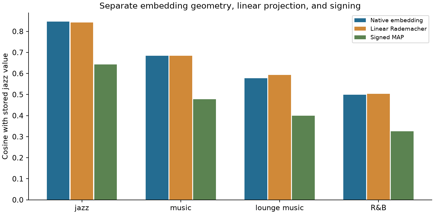
For lounge music compared with stored jazz, linear projection leaves their cosine similarity largely unchanged. The larger change occurs during signing: keeping only the sign of each component discards its magnitude, so the bipolar hypervectors retain the relationship with a lower similarity score.

For retrieval, this means we can carry the embedding model’s preference for better-matching phrases into HDC, so a query needn’t repeat the exact wording of a stored value.

E2: Retrieve a record with a phrase we never stored

We can now use the encoded query to ask: during retrieval, can the phrase lounge music rank Maya ahead of Nina (because only Maya has an interest that’s semantically similar to it)?

The query is encoded as follows:

We used LanceDB to store each person’s hypervector alongside their person_id, so we get back the projected columns we ask for, ordered by cosine distance. The returned ID lets us look up the original record to retrieve the full source data, including the full list of interests.

result = (
    table.search(unit(query).to(torch.float32).tolist())
    .distance_type("cosine")
    .bypass_vector_index()
    .limit(table.count_rows())
    .to_arrow()
)
rows = pl.from_arrow(result).to_dicts()
scores_by_id = {row["person_id"]: 1.0 - row["_distance"] for row in rows}

We test the exact stored interest, a related phrase, and an unrelated phrase:

As expected, Maya ranks first for lounge music. The exact wording jazz separates the records more strongly, even though its query encoding differs from the stored encoding. Moving to a related phrase broadens the matching evidence; it doesn’t guarantee equally clear discrimination.

The unrelated aircraft maintenance cue still gives both people scores near 0.30 and selects Nina.

This stage demonstrated how a bundled hypervector can support retrieval from a partial cue.

E3: Explain which facts contribute to the retrieval score

What drives Maya’s lounge music score: jazz, her other interests, or interference from age and eye color? To explain the retrieval score, we can unbind the interest role and examine the values contributing to the match.³ In HDC literature, this is called a role probe.

Comparing this role probe with the query value gives the same cosine score as the bound query’s search against Maya’s record. The experiment checks this equivalence across all 26 probes, with agreement within $10^{-12}$.

We then split Maya’s score into contributions from each fact, using the same normalization for all five so they add up to the original score.

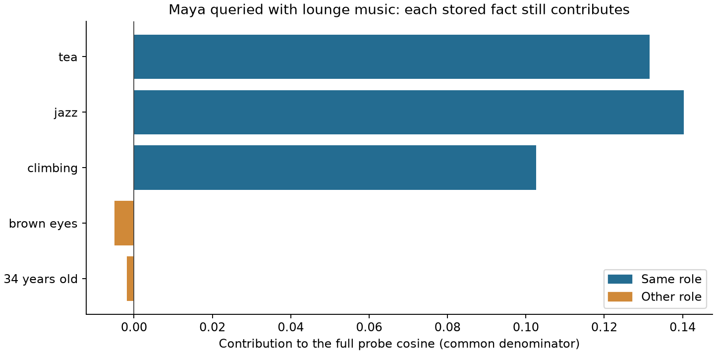
Jazz clearly contributes the most to the score, with tea and climbing also adding some of the evidence. Age and eye color remain in the interest probe: their interference is the crosstalk we introduced earlier, now measured to have little effect on this score.⁴

The additive structure of bundling lets us explain retrieval scores through individual source facts, unlike traditional embedding retrieval.

E4: Refine the query with positive and negative evidence

Both records contain a tea hypervector bound to the interest role and bundled with the other facts. To search for that shared interest, we encode tea as a query hypervector and bind it to the same role:

Suppose we now want to ask a query that favors tea drinkers but penalizes any evidence for the cue “brown eyes”. We can express that preference using the same additive structure of bundling:

Here, $\mathbf{h}_{\mathrm{refined}}$ is the refined query hypervector that indicates our preferences (not brown eyes). For each record, its dot-product score with the brown-eye query is subtracted from its score with the tea query, before cosine normalization. A stronger brown-eye match therefore subtracts more from the score. We expect this to penalize Maya more than Nina.

Subtracting the brown-eye query lowers Maya’s score more than Nina’s, moving Nina into first place. Maya still scores above zero because the refined query also matches other facts in her record.

This connects back to associative search over connected data ↗ . A graph might represent an interest as an edge; our HDC encoding represents it as a role-value binding. Similarity can propose a person from a partial cue, and the source record supplies exact properties and relationships for filtering and traversal.

This experiment showed how subtractive and additive bundling lets us combine positive and negative preferences at query time to refine retrieval without re-encoding the stored records.

E5: Test whether subtraction recovers the remaining bundle

This final experiment tests whether subtracting the jazz contribution from Maya’s bundle produces the same hypervector as encoding her remaining facts from scratch.

Bundling is additive, so subtracting the exact contribution for jazz should leave the sum of everything else. This is the prediction we test with $\mathbf{h}_{\mathrm{orange}}$, shown in orange bars in the chart below:

But lounge music is a similar cue that also closely matched Maya during retrieval. Does that similarity make it a valid substitute when subtracting? We test this with $\mathbf{h}_{\mathrm{green}}$, shown in green bars in the chart below:

We compare both results with Maya’s original bundle (blue) using four queries. Each group of bars shows the scores for one query. In particular, let’s focus on the middle cases, music and lounge music, from the chart:

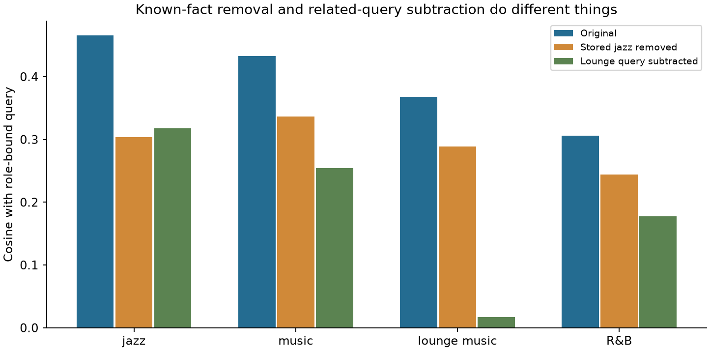
Semantic similarity lets us use similar phrases for retrieval, but those same phrases do not work well when subtracting from a bundle. The green lounge-music bar shows that subtracting this query leaves the resulting bundle with almost zero similarity to that same query.

The orange bars show that subtracting jazz from the full hypervector still lets us match the remaining evidence from tea and climbing. In E3, both interests contributed to the lounge music score alongside jazz. Subtracting jazz leaves those interests in the bundle, so that information remains in the bundle.

This experiment shows that we can remove a known exact fact from a bundle and maintain a high degree of similarity to the remaining facts, but we cannot remove a similar fact and expect the same result. The additive structure of bundling lets us subtract an exact contribution, but not necessarily a similar one.

Conclusions

Binding and bundling serve different purposes in HDC. Binding represents an association, such as an interest and its value, in a hypervector dissimilar to either input. Bundling represents a superposition of those associations so we can recognize their contributions through similarity.

Our experiments showed what the distinction between bundling and binding makes possible:

• Preserve semantic relationships: The tested phrases had different cosine similarity scores in text embedding space and HDC space, but retained their relative similarity ordering.
• Retrieve from a related cue: Lounge music ranked Maya first without an exact match to jazz. An unrelated query also produced a clear winner, so this showed how ranking alone didn’t establish relevance, but similarity guarantees a non-null result.
• Explain a score: Jazz, tea, and climbing all contributed to the lounge-music match. We could clearly measure and explain those contributions using the encoded source facts.
• Express query preferences: Subtracting evidence for brown eyes moved Nina above Maya in the tea search. It changed the ranking, without enforcing an exact exclusion.
• Distinguish removal from retrieval: The exact jazz contribution could be subtracted from the additive bundle. A related phrase could retrieve the record, but couldn’t substitute for that contribution when removing it.

You can reproduce these results using the code and instructions in the experiment repository ↗ .

When working with HDC, it’s natural to ask “Can bundling be reversed like binding?” This study shows why the more useful question for bundling is less about exact reversibility and more about recoverability: can we reliably recognize facts represented in the bundle? We don’t need to reconstruct every input to retrieve a relevant record or examine evidence for an attribute.

What we would study next

As more and more bound facts are added to a bundle, their contributions become harder to distinguish. The interesting next question becomes: how many facts can we bundle before we can no longer reliably identify which facts are present?

Our next study will vary the number of facts and hypervector dimensions in MAP, measuring how often constituent values can be identified correctly. We’ll compare categorical values with values that have a meaningful order, using nominal and ordinal encodings. This will show how bundling capacity changes with both dimensionality and the relationships between values.

These controlled encodings will help isolate the effects of superposition on how meaning is retained. The aim is to measure the point at which recovering facts becomes unreliable, rather than assume a universal number of facts that every bundle can hold. Stay tuned!