Where does meaning in a hypervector come from?

Random hypervectors in HDC give us reliably distinct starting points, while binding, bundling, and permutation let us compose them into richer representations. In this post, we’ll go one level deeper: how do we get hypervectors that are not just distinct, but also semantically similar when they should be?

High dimensionality alone doesn’t encode meaning ¹ into a representation. Because of the vastness of hypervector space, if we just created random 10,000-dimensional hypervectors for the concepts of cat, kitten, and volcano, all three would begin as nearly orthogonal patterns. The geometry may be useful, but it doesn’t know that a cat and a kitten are semantically related concepts.

As anyone who’s worked with semantic similarity in natural language processing (NLP) would know, inputs that are related for a task should be closer than unrelated inputs.

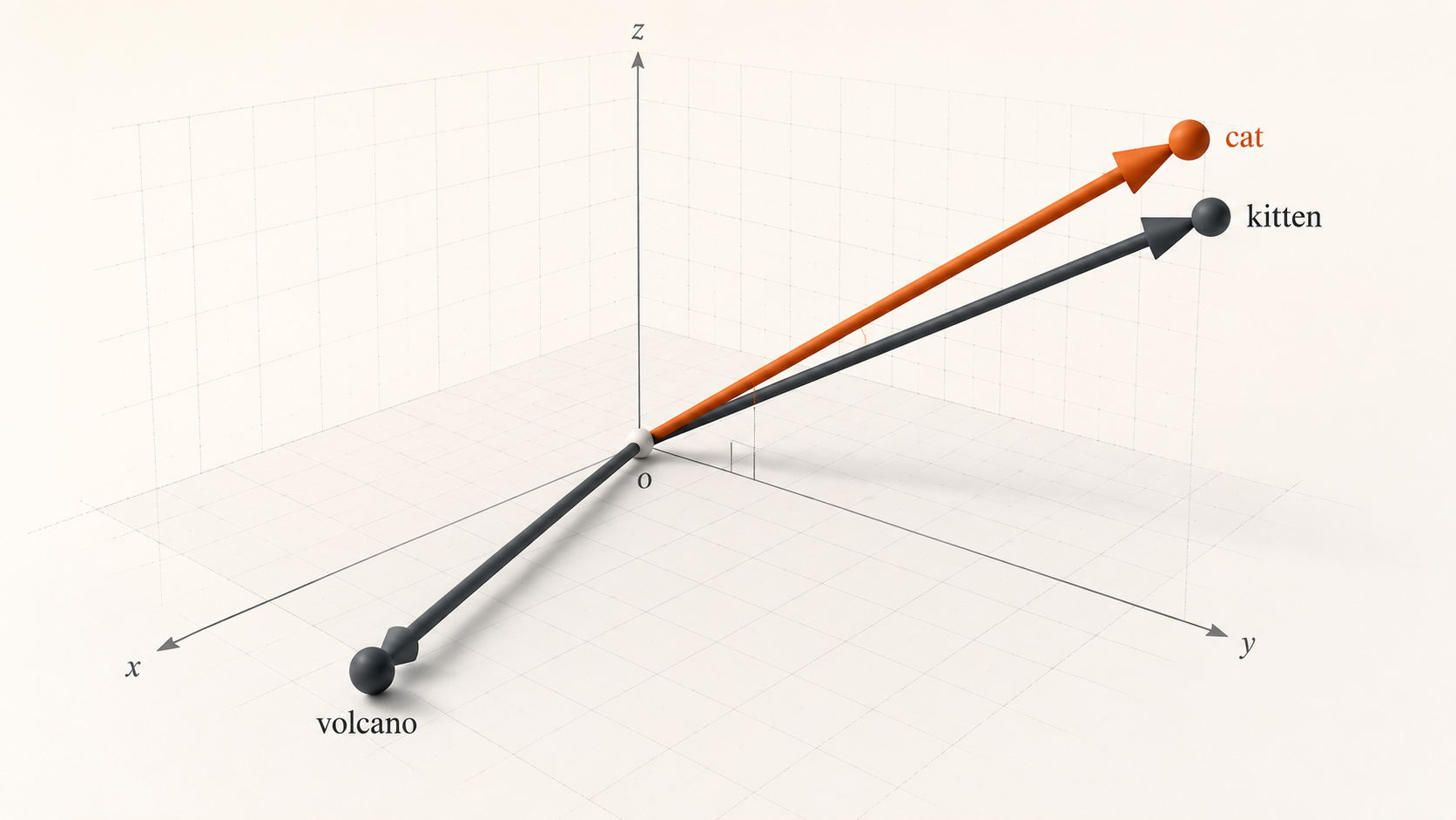
This shifts the problem from whether a hypervector somehow contains “meaning” to a more precise design question: which relationships should an encoder preserve, and where does that similarity structure come from? We’ll compare random codebooks, random projections from learned embeddings, and then test what survives when a learned embedding is projected into hypervector space.

The classical approach: random codebooks

Classical HDC/VSA usually starts with a codebook: the first time we encounter a symbol, we generate a random hypervector and store the pair. Every later lookup of that symbol returns the same hypervector.

codebook = {
  "cat":     random_hypervector(),
  "kitten":  random_hypervector(),
  "volcano": random_hypervector()
}

This is simple and effective for a small, fixed vocabulary. However, the codebook needs one stored hypervector for every distinct symbol. For a vocabulary $V$ and hypervector dimensionality $D$, storage grows with $|V| \times D$. An open-ended collection of words, phrases, products, or entities can therefore produce a very large codebook, along with a vocabulary that has to be kept consistent as new items arrive.

Much of the foundational HDC/VSA work, including Pentti Kanerva’s 2009 introduction, ² predates the transformer architecture and modern models designed to produce reusable embeddings.

Today, learned representations like semantic embeddings (commonly used in retrieval-augmented generation, or RAG, systems) let us start with useful relationships already encoded in the geometry. We can bring that structure into HDC in two ways:

1. Project a pretrained embedding. A fixed random matrix carries its existing similarity structure into hypervector space, without training a new encoder.
2. Learn a representation for the task itself. Training shapes the hypervectors directly around the relationships needed by the downstream task.

Let’s see how this works in the sections below.

Random projection preserves more than you might expect

Suppose we begin with a semantic embedding:

$$x \in \mathbb{R}^{768}.$$

The individual coordinates are not especially meaningful by themselves. What matters is the geometry of the space they collectively define. If the embedding model has done its job well, semantically related concepts already point in similar directions, while unrelated concepts are farther apart.

So when we move into a 10,000-dimensional hypervector space, we don’t want to learn semantics all over again. The embedding model has already done the hard part. Our goal is simply to re-express that geometry in a much larger, distributed representation.

One way to do that is with a fixed random Rademacher matrix ³ :

$$R \in \{-1,+1\}^{768\times10{,}000}$$

This lets us compute:

$$h=xR$$

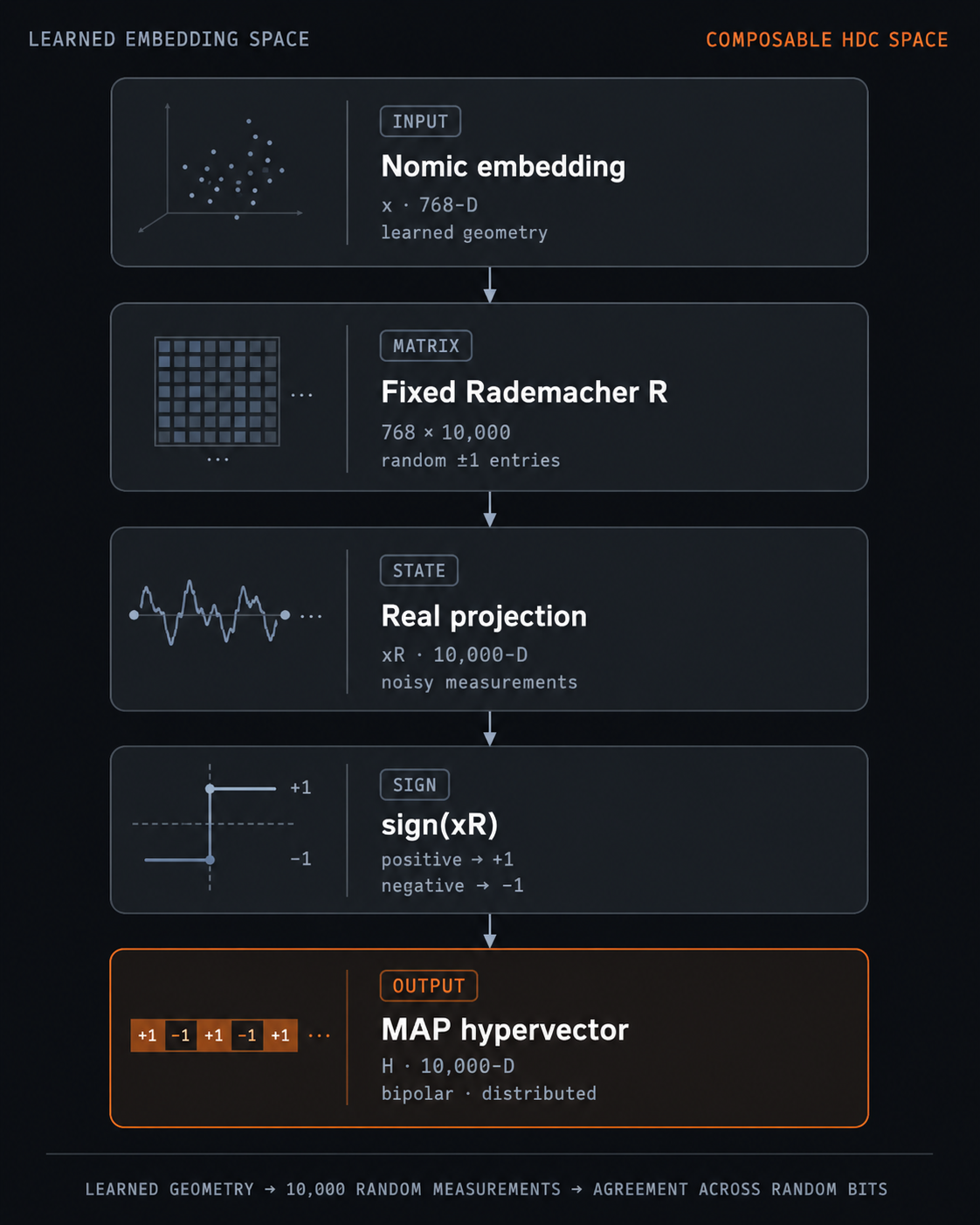
Multiplying a $1\times768$ Nomic text embedding by a $768\times10{,}000$ Rademacher matrix returns a $1\times10{,}000$ array, exactly the dimension we need for our hypervector space.

Each output value in the resulting hypervector is a different random mixture of all 768 input dimensions. The random matrix is essentially acting as a giant semantic mixer.

$$h_j=\sum_i x_iR_{ij}$$

No individual coordinate corresponds to a concept like cat, animal, or volcano. The learned structure is distributed across the full 10,000-dimensional pattern instead, giving HDC a representation whose identity lives in the whole pattern. Importantly, each entry in the matrix is sampled once from a Rademacher distribution, and the matrix is then fixed. Every embedding goes through the same random transformation.

However, the result of $h=xR$ is still a real-valued hypervector with 10,000 dimensions. Let’s see how we can turn it into a bipolar hypervector that HDC can work with using MAP.

From real-valued to bipolar hypervectors

A MAP encoder applies the sign function to every projected value of the hypervector:

$$H=\operatorname{sign}(xR)$$

giving us:

$$H\in\{-1,+1\}^{10{,}000}$$

This is a nonlinear quantization step. A useful way to visualize it is to treat each column $r_j$ of $R$ as a random hyperplane through the origin. The corresponding output bit at each position can be computed as follows:

$$H_j=\operatorname{sign}(x\cdot r_j)$$

This is like asking a simple yes-or-no question: On which side of this random hyperplane does $x$ lie? Each coordinate records one answer. A 10,000-dimensional bipolar hypervector records 10,000 of them. This matters because no single arbitrary split carries much weight in the final representation. ⁴

Two very similar embeddings pointing in similar directions, such as “cat” and “kitten,” will land on the same side of most of those hyperplanes, so their bipolar hypervectors will contain many matching signs. Two nearly orthogonal, or highly dissimilar, embeddings will agree only about half the time. After this step, semantic similarity has become agreement across thousands of random bits.

The figure below summarizes the sequence of steps that transforms a 768-dimensional embedding into a 10,000-dimensional bipolar MAP hypervector.

HDC provides the algebra

A text embedding model learns the structure of language from data: which points are nearby, which directions are similar, and which regions of the space are far apart. In other words, semantic similarity is expressed through the geometry and topology of relationships across the space, but that structure is opaque and hard to inspect.

In HDC, we want to do more than compare representations by similarity; we want to operate on the representations algebraically. We want to bind concepts to roles, bundle them into larger representations, and impose structure such as position or order. But those operations require the text representations to inhabit the same high-dimensional space as the rest of our hypervectors, where HDC’s distributed and compositional properties emerge.

The upward projection gives us that compatibility:

$$\mathbb{R}^{768} \longrightarrow \{-1,+1\}^{10{,}000}$$

If two concepts were close before projection, we want them to remain close afterward; if they were unrelated, we want that separation to remain visible.

This is exactly what we achieved through random projection: we take a lower-dimensional representation whose semantics are already encoded in its geometry and move it into a space where those semantics can participate in HDC’s compositional algebra.

HDC can then operate on representations that preserve those semantic relationships and can also be composed, transformed, and explained.

Does this work in practice?

Let’s test the idea with actual values by generating unit-normalized embeddings using a locally running Ollama nomic-embed-text model. ⁵ All three text embeddings are then passed through the same Rademacher matrix and the sign function. For reproducibility, the random matrix is seeded with a fixed value.

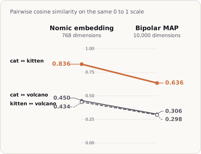
The most important takeaway from this experiment is that the learned similarity in a lower-dimensional text embedding was successfully transferred to a higher-dimensional space, in a form that HDC can operate on.

Can the hypervectors themselves be learned?

So far, we have treated randomness as a useful starting point for HDC. But that doesn’t mean every hypervector must be random or that we have to transfer semantic information from a pretrained embedding.

Recent work ⁶ has started to make different parts of the HDC pipeline learnable. Some approaches learn the class hypervectors instead of constructing them only by bundling examples. Newer work goes further and learns the base hypervectors used by the encoder, allowing the task data to shape the representation itself.

Conceptually, the distinction is simple:

• Fixed projection carries a similarity structure learned elsewhere into hypervector space.
• Learned HDC allows some of that structure to be shaped directly inside hypervector space.

Both point to the same broader idea: high dimensionality gives us the representational canvas, but it does not decide what the geometry should mean. That comes from the encoder, the data, or both.

Conclusions

This post examined the different ways semantic similarity can enter hypervector space. The key takeaways are:

1. High dimensionality provides the canvas, not the semantics. It makes unrelated hypervectors reliably distinct, leaving room for useful similarity to stand out.
2. The encoder determines where similarity comes from. A codebook treats symbols as independent, a pretrained embedding brings relationships learned from data, and a learned HDC encoder can shape those relationships for a particular task.
3. Projection provides a bridge between learned geometry and HDC algebra. It can carry useful neighborhood structure into a compatible hypervector space, where binding, bundling, and permutation can add roles, collections, and order.

This is why modern HDC is starting to look less like an alternative to the rest of machine learning and more like a natural partner. Deep learning is remarkably good at learning useful similarity structures from complex data. HDC gives us a high-dimensional, distributed algebra for composing those representations once we have them. As recent work on learnable hypervector representations shows, ⁶ that boundary is becoming even less rigid.

In the next post, we’ll look more closely at the parallels between HDC and deep learning, along with the important differences in how they learn, represent, and operate on information. The interesting question isn’t whether one replaces the other, but what becomes possible when we let each approach contribute what it does best.

Footnotes

1. In this post, semantic similarity means measurable proximity between inputs based on relationships learned from a model’s training signal. We use the term “meaning” here more informally: we don’t mean that the model possesses human-like understanding. Emily M. Bender and Alexander Koller distinguish linguistic form from meaning (the relation between form and communicative intent) and argue that a system trained only on form cannot learn meaning from form alone. See “Climbing towards NLU: On Meaning, Form, and Understanding in the Age of Data”↗ , Proceedings of the 58th Annual Meeting of the Association for Computational Linguistics (2020): 5185–5198. ↩

2. Pentti Kanerva, “Hyperdimensional Computing: An Introduction to Computing in Distributed Representation with High-Dimensional Random Vectors”↗ , Cognitive Computation 1 (2009): 139–159. ↩

3. A Rademacher matrix has entries sampled independently from a Rademacher distribution, so each entry is $+1$ or $-1$ with equal probability. Once sampled, the matrix is fixed and reused for every embedding. ↩

4. Moses S. Charikar, “Similarity Estimation Techniques from Rounding Algorithms”↗ , Proceedings of the 34th Annual ACM Symposium on Theory of Computing (2002): 380–388. The key result for our purposes is that a random hyperplane gives two vectors the same sign with probability $1 - \theta / \pi$, where $\theta$ is the angle between them. Similar vectors therefore agree on more bits, while orthogonal vectors agree about half the time. ↩

5. Ollama, “nomic-embed-text”↗ . The current Ollama model metadata shows that it’s a 768-dimensional text embedding with mean pooling. ↩

6. LeHDC↗ learns class hypervectors while keeping the encoder and inference procedure fixed. More recent Trainable Hyperdimensional Computing (THDC)↗ learns both the base hypervectors used by the encoder and the class hypervectors together. Both are classification-focused examples, but they illustrate how learning can move progressively deeper into the HDC pipeline. ↩ ↩²