
Why connected data needs associative search
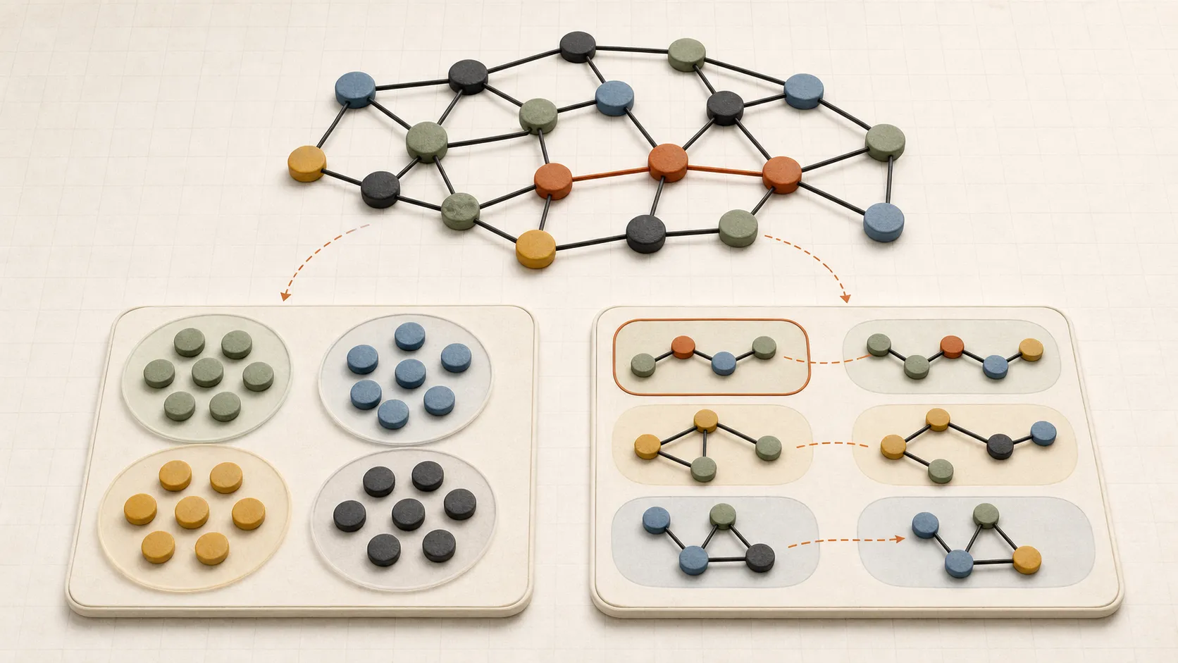
Graph search follows exact relationships, while associative search finds similar situations from incomplete examples.

On this page
In earlier posts, we’ve seen how HDC can encode structure in data. Once encoded as hypervectors, connected structures can be compared and ranked by similarity. In this post, we’ll cover associative search, where we begin with a relevant candidate and find others that resemble it.
Let’s imagine a retail dataset with sales orders, the items they contain, the customers who placed them, and the addresses where they were shipped. An analyst might know the sales order ID, which gives us a place to start: find the order, then join or traverse outward to its line items, shipping address, and customer.
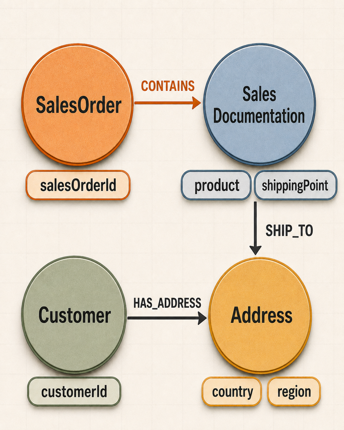
Most queries over structured data like this begin with an exact query in SQL or Cypher. Given a salesOrderId, the Cypher query below follows the exact relationships to its items, shipping address, and customer.
MATCH (order:SalesOrder { salesOrderId: $salesOrderId })
      -[:CONTAINS]->(item:SalesDocumentItem)
      -[:SHIP_TO]->(address:Address)
MATCH (customer:Customer)-[:HAS_ADDRESS]->(address)
RETURN order, item, customer, address
Property graphs and exact traversals are fantastic when we know what we want because they turn those relationships into labeled, directed edges that we can follow and inspect.
What if the pattern is the query?
Investigative work often begins in the opposite direction. We notice a connected graph pattern before we know which properties we care about. In this example, the pattern is not a single entity or path: it’s a three-edge motif.1
An order contains an item, the item ships to an address, and a customer has that address. Instead of an exact match, our question may look more like this:
This pattern looks interesting. Show me other patterns that are similar to this.
Similarity could depend on shared topology, the direction and role of each relationship, or selected properties such as product, region, and shipping point. Each interpretation implies a different scoring rule. We’ve quietly moved from asking whether an exact graph pattern exists to asking how much relational structure and property information two records share.
Cypher can express that search, but the similarity logic has to be made explicit through shorter patterns, optional matches, predicates, weights, or scoring branches. Explicit Cypher scoring is reasonable when we already know the variations that matter. When an incomplete example is the best query we have, it means defining every acceptable completion and score before retrieval.
Associative search works with incomplete information
Here, “associative search” means using the information we have to look for related, complete records. The known relationships and property values are encoded as a query hypervector, compared with the stored hypervectors, and ranked by similarity. A lookup key, such as an order ID, can then map each result back to the explicit entities and relationships in the graph.
In our example, the three-edge schema is already known. What may be incomplete are the property values. We might know the address country and the item’s shipping point, but not the address region:
A highly ranked result can still point back to a complete graph record whose Address contains the missing region. The search does not infer that value; it retrieves a stored pattern whose graph record already contains it.
The word “associative” doesn’t imply that the system discovers every connection that may be meaningful. Associative retrieval compares stored information with the query instead of looking it up with a record identifier. There are three important differences between associative search and exact graph search:
- The searchable unit is an encoded graph pattern, not an isolated node record
- The query can omit property values that are unavailable
- The result is a set of candidates ranked by similarity scores, so they are likely (but not guaranteed) to be relevant
Searching with incomplete information is useful in investigative work. We can begin with a situation we’ve observed before we have an exact identifier or a complete set of matching fields for locating it exactly.
What about traditional vector search?
At this point, traditional vector search, as commonly used in retrieval-augmented generation (RAG), looks like a viable alternative to HDC and associative search. If exact matches are too restrictive, why not embed each customer, product, or address and retrieve the nearest ones?
An entity-level embedding is useful when the entity is the thing we want to compare. Two customers may be close because a learned embedding places their names, descriptions, or other properties in the same semantic neighborhood. However, that proximity doesn’t tell us what role each entity plays in the graph around it.
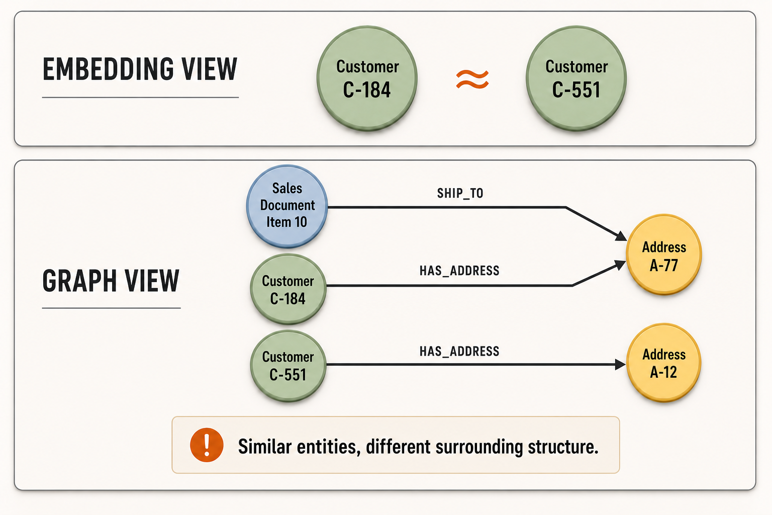
The distinction between traditional vector search and associative search lies in the representations, not the retrieval mechanisms. Both approaches can use vector similarity for retrieval. The difference is what we choose to encode: in HDC, each hypervector can combine several directed relationships, allowing similarity to reflect shared relational structure rather than entity metadata alone.
A traditional embedding model could be used to embed the textual metadata of an entity, such as a sales order’s description, but this doesn’t capture the relational structure. Simply traversing outward from a retrieved entity does not make that structure part of the similarity score.
Modeling connected data in HDC
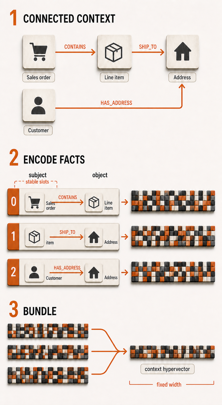
The HDC operations we’ve already introduced let us encode a graph pattern in two steps: represent each directed relationship as a subject-predicate-object fact, then bundle the three fact hypervectors into one.
Suppose fact has subject entity , predicate , and object entity . The entity hypervectors and can encode their types and any selected properties that should affect similarity:
Binding preserves the direction of each relationship, so swapping the subject and object changes its encoding. Here, the three facts are SalesOrder CONTAINS SalesDocumentItem, SalesDocumentItem SHIP_TO Address, and Customer HAS_ADDRESS Address. The term applies a different permutation to each fact, keeping the three encodings distinct when they are combined.
Bundling then produces one hypervector for the complete graph pattern:
What we include in each entity hypervector determines what the resulting pattern hypervector can distinguish:
- If the entity representations include only node types, such as
SalesOrderandCustomer, every record with this typed motif produces the same pattern hypervector. The representation can retrieve a structural template, but it cannot rank individual sales records against one another. - Distinguishing individual records requires properties, timestamps, or semantic features that vary across instances. The index can retain IDs such as
SO-1042andC-184for graph lookup without making those arbitrary identifiers part of the similarity measure.
Similarity can degrade gradually as information is removed
Associative search is useful because similarity can degrade gradually as property values are removed from a query. The behavior mirrors an investigative scenario in which an analyst recognizes the shape of an interesting motif but does not know every field needed for an exact query.
Let represent the motif we want to study. Each term below represents one directed relationship, including its endpoint types and relationship label.
For this example, each selected property contributes one role-bound component to the hypervector. Let , , and represent the encoded property values bound to their respective keys. The complete hypervector then bundles all six components:
Let’s assume that MAP bundling uses element-wise addition and that these six components are unit-length and nearly orthogonal.2
An ideal query contains the entire motif and all its required property values. In a graph, those inputs can provide an exact match. In HDC, the query hypervector is identical to the complete hypervector, giving a similarity score of 1.00:
In a more realistic investigative scenario, the address country and shipping point are known but the region may not be. The query hypervector then omits only :
Even if both the region and shipping point are unknown, the query still retains the overall structure and the known country, providing a useful similarity score:
Each missing property weakens the similarity score without changing the graph pattern being searched. We call this behavior graceful degradation: incomplete inputs can still retrieve candidates instead of becoming pass-or-fail filters.
The Cypher query below retrieves the same three-edge motif while allowing for missing property values. Nullable parameters handle cases in which the region or shipping point is unknown:
MATCH (order:SalesOrder)-[:CONTAINS]->(item:SalesDocumentItem)
      -[:SHIP_TO]->(address:Address)
MATCH (customer:Customer)-[:HAS_ADDRESS]->(address)
WHERE address.country = $country
  AND ($region IS NULL OR address.region = $region)
  AND ($shippingPoint IS NULL OR item.shippingPoint = $shippingPoint)
RETURN order, item, customer, address
The Cypher query handles missing inputs, but each known value remains an exact predicate. Supporting graded partial matches would require explicit scoring logic for the properties we want to compare.
HDC proposes, graph validates
Once we encode a connected graph pattern as a hypervector, we can search using the pattern itself. A human analyst or AI agent no longer has to reduce an observed situation to a record ID or a fully specified set of predicates. The relationships and property values they do know become the query; HDC retrieves similar stored patterns, and the index leads back to the exact graph records.
The resulting workflow creates a natural separation of responsibilities. HDC and associative search propose candidates, while the graph validates them. The graph contains the exact facts, while HDC ranks connected graph patterns that are similar enough for a human or agent to investigate further.
Combining associative search with graph validation raises a broader question: what becomes possible when approximate search can coexist with the exact graph in a real-world application?
Where we go from here
Connected data is useful precisely because it explicitly models relationships. Exact graph traversals can expose the relevant facts once we know which patterns to inspect. Associative search can be beneficial when the connected graph pattern itself is the best query we have.
We believe connected data needs associative search for discovery because it lets us move from records we can name to situations we can recognize. The graph preserves what’s connected, and HDC makes the graph pattern itself searchable. Together, they add a retrieval layer while preserving the graph’s explicit structure.
This post presented a design argument, not a concrete implementation. Future posts will test the approach across practical use cases by encoding graph patterns as hypervectors and measuring how incomplete queries, encoder choices, and crosstalk affect retrieval. Stay tuned!
Footnotes
-
Strictly, network motifs are recurring patterns of interconnections that appear more often than in randomized networks, as introduced by Milo et al. A graph pattern is the broader term for any arrangement used for matching. We use motif here informally for the three-edge shape, not as a claim of statistical significance. ↩
-
For a stored bundle of nearly orthogonal unit components, the bundle’s norm is approximately . If a query retains of those components, their dot product is approximately and the query norm is , giving cosine similarity . The one-component case reduces to . ↩