
Turn graph data into hypervectors for associative search
Learn how to encode node properties and edge direction with HDC, compose a partial query, and resolve similarity matches back to exact graph records.

On this page
A property graph makes relationships explicit: we can see who is connected to whom, how they’re connected, and what we know about each entity. From an associative search perspective, this raises an interesting question: how can we make the properties and relationships retrievable, even when we have partial information?
In our earlier post on why connected data needs associative search, we explored using an incomplete description to find related, complete graph records. Here, we’ll work through how to build an alternate representation of the nodes and relationships in the graph using HDC.
The central idea is to bind each property into the representation of a node or a relationship, and then bundle those contributions into a single hypervector that represents a path. The resulting hypervector can be compared with others to find similar records, even when the query doesn’t specify every property.
The best way to see this in action is to work our way through a simple graph. We’ll follow node and relationship properties into a searchable path hypervector, build a query from a few remembered details, and trace the result back to the original graph. Along the way, we’ll see why leaving information out when querying in HDC can still produce a useful match, and where it introduces ambiguity.
Start with a simple graph
Let’s use our familiar friends Maya and Nina, who appeared in our post on bundled hypervectors. In this post, we’ll keep their properties and extend their story to form a small graph. Let’s assume Maya mentors Nina on a weekly basis, and that Nina works full-time at a robotics organization in Toronto called Cedar Lab.
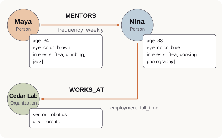
The path has three nodes and two directed edges: (Maya)-[:MENTORS]->(Nina)-[:WORKS_AT]->(Cedar Lab). Nina is the bridge in the path between Maya and the organization Cedar Lab.
The properties belong to different parts of this path. The eye_color property describes a Person, while the frequency property describes how often the MENTORS relationship occurs. Nina’s employment arrangement belongs to her WORKS_AT edge; Cedar Lab’s sector belongs to the organization itself.
Now consider a path-like search query:
Find a tea drinker who mentors someone who is interested in cooking.
What’s interesting about this query is that it’s inherently directional. A tea drinker mentoring someone interested in cooking is a different arrangement from someone interested in cooking mentoring a tea drinker. The query also specifies only a few properties in the path: it doesn’t mention ages, eye colors, or the organization’s city. As we retrieve results, we’ll see how the HDC approach to associative search compares this partial description with complete paths, using the properties and their positions together.
Turn nodes into hypervectors
In HDC, we represent information using hypervectors, which are long arrays of numbers, typically with thousands of dimensions. In this post, we pick a fixed dimensionality of 4,096. A fact like “Nina has blue eyes” is spread across the entire hypervector, rather than assigned to a single position reserved for tea or eye color.1
The raw data is turned into hypervectors using an encoder. The encoder maps each role and value to a unique hypervector, and then combines them using the three operators of HDC: binding, bundling, and permutation. The resulting hypervector is a single representation of a collection of facts about an entity, or as we’ll see below, a path through the graph.
To encode the fact that Nina has blue eyes, we bind a role eye_color (a string) to the value blue (also a string). Each of these is an independent random bipolar hypervector, and we bind them by multiplying them element-wise.2 The image below shows the first ten components of the two hypervectors and their product. The result is a new hypervector that represents the fact “Nina has blue eyes.”
In the same way, we encode age: 33, where the value 33 is a number that has its own unique hypervector. The two role-value hypervectors for the eye color and age are then bundled together to create a single new hypervector that represents the combined facts. Note that in the image below, the inputs are the two bound role-value hypervectors for Nina’s age and eye color.
Going through a similar process for the remaining facts, we can bundle all of Nina’s properties into a single hypervector, :
The hypervector for Maya () is also generated using the same encoding process: in her case, with an age of 34, brown eyes, and interests in tea, climbing, and jazz. Both persons in this dataset have a common interest in tea, encoded as . This means that a query about “tea” should return matching evidence from both bundles.
Query an entity hypervector
We’ve encoded the properties of a Person node in the graph, representing an entity. In this section, we’ll see how to retrieve that entity from a partial description, using the same binding and bundling operations.
The query below binds the eye_color role to the blue value, producing a query hypervector, :
We’re querying with a partial cue: only eye_color: blue. We compare its hypervector with the hypervectors in the persons table using cosine similarity, without filtering on eye color. Nina’s age and interests don’t need to be specified.
Running the companion example with TorchHD, LanceDB, and 4,096-dimensional categorical hypervectors gives these results. The vocabulary uses a fixed random seed of 2026, and scores are rounded down to four decimal places.
| Rank | node_id | Stored hypervector | Cosine similarity |
|---|---|---|---|
| 1 | nina | 0.4566 | |
| 2 | maya | -0.0062 |
Nina ranks first because her bundle contains the bound blue-eyes fact. Maya’s score got pushed away from 1 because she has brown, not blue eyes. Once we retrieve the full bundled hypervector for a Person entity through the similarity search, we can fetch the full record from the LanceDB database by looking up her node_id.
What if we also want our query to include the person’s interest in cooking? We can compose it to the eye color component with bundling, as follows:
| node_id | Blue eyes only | Blue eyes + cooking |
|---|---|---|
nina | 0.4566 | 0.6328 |
maya | -0.0062 | 0.0084 |
The top result is once again Nina, with her score rising from 0.4566 to 0.6328, because the query now shares two bound facts with her stored hypervector. Maya’s score remains close to zero. Even though we used a partial description of properties of the entity, we were able to retrieve a relevant entity via similarity search.
Say we now change the cue to brown eyes. The ranking immediately flips: we see Maya appear as the top result:
| Rank | node_id | Stored hypervector | Cosine similarity |
|---|---|---|---|
| 1 | maya | 0.4396 | |
| 2 | nina | -0.0078 |
Throughout the query process, the stored hypervectors haven’t changed. We can compose arbitrary queries that aim to find relevant roles and their values from the data that’s stored in hyperspace.
Turn paths into hypervectors
So far, the queries we asked retrieved entity-level information. However, our opening query asked for information that’s in a path: we’re looking for properties that contain tea and cooking (in nodes), along a mentorship relationship.
In a property graph, this would be a straightforward Cypher traversal: we can follow the MENTORS edge from a tea drinker to a cooking enthusiast. In hypervector space, we’d need to encode the same information in a single representation for the entire path.
Encode a path hypervector
First, we create a hypervector that represents the Organization node for “Cedar Lab”. Similar to the process described above, we bind its sector and city roles to their property values and then bundle them:
In property graphs, relationships can carry properties too. Our source data here has relationship properties, so we give each relationship the fixed role type, bind its hypervector to the respective value, and then bundle it to other bound role-value pairs:
To store each relationship as a one-edge path, we combine its source node, relationship properties, and target node. However, in combining them, we must preserve the query’s semantics: the order matters: “who mentored whom?” Naively bundling the person hypervectors would erase that order, giving the same result if Maya and Nina exchanged places.
We use permutation to give each node and relationship a position before bundling.3 Here, is a one-element cyclic shift: move every component one place to the right, wrapping the last component around to the first. Applying it twice, , shifts by two places.
Each cyclic shift moves the same values to new positions. The teaching example wraps after ten components; our stored hypervectors wrap at their full dimension.
Each one-edge path uses the same positions:
Maya → MENTORS → Nina       Nina → WORKS_AT → Cedar Lab
  0       1       2          0        1          2
Position 0 stays unchanged, position 1 shifts once, and position 2 shifts twice. We apply this convention to both relationships:
We store nodes in persons and organizations, and these one-edge path hypervectors in mentors and works_at. Each relationship row retains its endpoint IDs and original edge properties. The partial values below are illustrative.
Persons (persons)
| node_id | name | label | hypervector |
|---|---|---|---|
maya | Maya | Person | : [+1, -1, +3, ...] |
nina | Nina | Person | : [-1, +3, +1, ...] |
Organizations (organizations)
| node_id | name | label | hypervector |
|---|---|---|---|
cedar | Cedar Lab | Organization | : [+2, 0, -2, ...] |
Mentoring relationships (mentors)
| edge_id | source_id | target_id | hypervector |
|---|---|---|---|
mentoring_1 | maya | nina | : [+2, -4, 0, ...] |
Employment relationships (works_at)
| edge_id | source_id | target_id | hypervector |
|---|---|---|---|
employment_1 | nina | cedar | : [+1, -3, +1, ...] |
Query a path hypervector
We can now follow the same approach as the blue-eyes query: encode only the facts we know, then compare the query with stored hypervectors. The extra step is to put each fact in its requested path position.
Returning to our original request:
Find a tea drinker who mentors someone who is interested in cooking.
The query above can be decomposed into role-value (entity) and relationship components. Each subquery is created by binding the roles with their respective values.
The query we need is a path of length 1, so with just two permutation shifts, we can encode the query’s order directly into its hypervector. The first component of the path, , stays unpermuted, is permuted once, and is permuted twice. Using the stored path’s positional convention gives these facts the meaning we want: the tea interest is in the first position, the mentoring relationship is in the second, and the cooking interest is in the third.
This one-edge query searches the mentors table directly in LanceDB. The result identifies the stored mentoring relationship, with its source and target IDs:
| edge_id | source_id | target_id | Stored hypervector |
|---|---|---|---|
mentoring_1 | maya | nina |
Looking up these IDs retrieves the mentoring record and both people from persons. The query supplied only their interests and the relationship type; the records include their other properties too.
Find similar paths from a shared pattern
Our partial query led us to a complete path without naming Maya or Nina. The same description can also match paths involving entirely different people. Once properties and relationships are composed into a hypervector, we can search for similar paths, not just similar entities.
Imagine adding Omar and Pedro to the graph: Omar mentors Pedro, Pedro likes cooking, and Pedro works at Cedar Lab in Toronto. We now have two pairs of people connected through the same pattern:
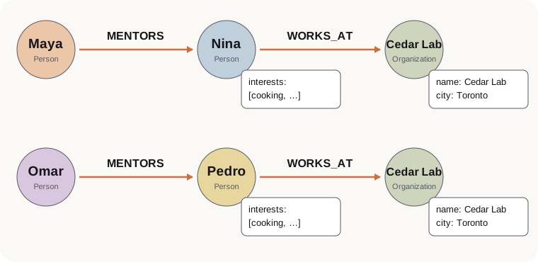
We can ask a new pattern query:
Find me people who mentored other people who work at Cedar Lab in Toronto. The person being mentored likes cooking.
This query leaves the mentor’s properties open. It specifies a mentee’s interest, two directed relationships, and the employer’s name and city. We can compose it using the same algebra, choosing a different set of facts from the path.
To search by the employer’s name, we first include that property in Cedar Lab’s stored hypervector. Its earlier bundle contained only sector and city; we add and rebuild the one-edge employment hypervectors that include it. The query’s employer contribution then binds just the name and city:
We reuse the mentoring and cooking cues from the previous query, omit tea, and add employment and the employer at their path positions:
There is no contribution at position 0 because we haven’t specified any mentor properties. The cooking cue still belongs to the mentee at position 2, and Cedar Lab’s name and city belong to the employer at position 4.
To find two-edge candidates, we join mentors.target_id to works_at.source_id. For Maya and Nina, composition is:
Shifting the employment hypervector twice places Cedar Lab at position 4. Both edges now contribute Nina at position 2, so we subtract one copy. With our unthresholded sums, this gives the same five-position path as encoding all its parts together.4
We compose and score these candidates in memory using TorchHD; LanceDB holds the reusable one-edge records. Both candidates contain the requested facts at the right positions. Their ordered edge IDs identify the results, without a stored path_id:
| node_ids | edge_ids | Matching pattern |
|---|---|---|
[maya, nina, cedar] | [mentoring_1, employment_1] | Mentor → cooking enthusiast → Cedar Lab, Toronto |
[omar, pedro, cedar] | [mentoring_2, employment_2] | Mentor → cooking enthusiast → Cedar Lab, Toronto |
These are illustrative matches, not measured rankings. The people’s other properties can differ and affect their similarity scores; the query’s shared evidence is the relationship pattern and the selected facts within it. The graph supplies the Person labels and verifies that each mentee is also the employee connecting the two edges.
The path query is composable. We choose which encoded properties matter, bind them to their roles, shift them into their path positions, and bundle the result. Changing the question changes those contributions; the same similarity operation still retrieves complete paths. Properties we never encoded must first be added to storage, as we did with the employer’s name.
This is the associative-search idea from our earlier post: a partial description can retrieve connected records that share a pattern, even when they involve different people. We can describe the relationships we care about without knowing every entity in advance.
From partial cues to connected patterns
Looking at all the steps above, you might come up with a natural question: “Why HDC? Can’t I simply answer queries with partial cues in a Cypher query instead?” The problem isn’t with Cypher: it’s that the strict need for exact matching in Cypher is less forgiving when even a single value differs (but is semantically similar). This is what leads to the entire MATCH query returning a null response.5
Because HDC does similarity search, it always returns results, while also allowing related terms (e.g., synonyms) to contribute to the same pattern query. For this, we replace the relevant random value hypervectors with projected semantic embeddings, baking it into the design of the encoder at both storage and query time.
Let’s look at an interesting example where HDC shines. Say our query asked for people with an interest in baking, but the stored path contains an interest in cooking:
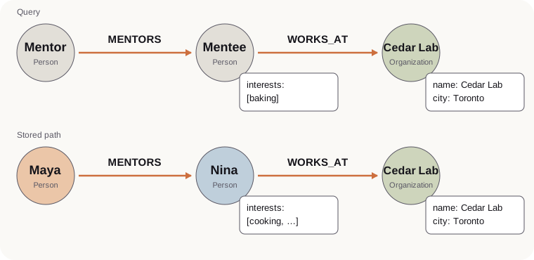
An exact Cypher query that used the term baking as a property filter would exclude Nina’s path, returning no results. However, our HDC encoder can represent “baking” and “cooking” as similar, binding both to interest and, with permutation, retaining the fact that a term similar to cooking is at the mentee’s position in the path. The HDC version of this query would return the path for Nina, even though the stored path doesn’t contain the exact term “baking”.
The same applies to relationships: a query that asks for persons EMPLOYED_AT an organization doesn’t literally match the graph’s WORKS_AT relationship, so an ordinary Cypher query with that explicitly named relationship would return nothing. However, in HDC, we encode the predicate the same way we encode string values in node properties, via binding. So it can capture semantic similarity in the relationship labels themselves, not just properties.
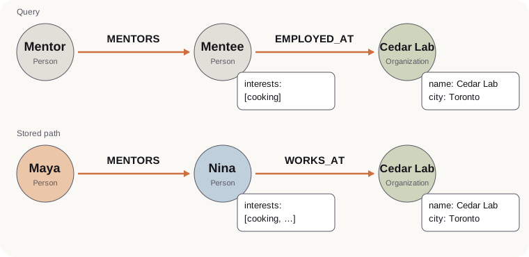
In HDC, binding, bundling, and permutation let us compose queries for similar patterns, not just similar entities. Exact-value cues and semantic cues can both be part of the same query, over an entire path. Top-k returns the nearest available candidates even without an exact match, provided the candidate set isn’t empty and no score cutoff excludes them. Importantly, these queries can be composed at query time, without precomputing every possible n-hop path. We simply need to encode the relevant facts upfront in the relationship tables (for one-edge paths) and then compose them at query time for longer paths of length .
This suggests a fascinating direction to explore in future posts: which parts of a query should be guided by similarity-based retrieval, and which should remain exact matches? HDC could propose plausible candidates by identifying and surfacing interesting patterns, while exact graph traversal validates required facts and follows further connections. Together, they could help agents work from incomplete descriptions while keeping their answers tied to explicit records that we can validate.
Code
You can work through these examples in the code repository, with step-by-step lessons for encoding nodes and relationships, composing paths, and creating composable queries for similarity search using TorchHD and LanceDB.
Footnotes
-
This is the holographic property: information is distributed across the hypervector, so the overall pattern represents a fact rather than any single component. See our earlier article, The Holographic Nature of Hypervectors, for how this distribution helps representations remain recognizable when some components are missing or altered. ↩
-
TorchHD’s MAP documentation defines binding as element-wise multiplication, bundling as element-wise addition, and permutation as rearranging components to encode order. We keep bundles as unthresholded sums and reuse the same vocabulary and positional shifts in storage and queries. ↩
-
See Why permutation matters in HDC for an introduction to the operation and why it preserves structure. ↩
-
The example enumerates connected edge pairs before scoring. Larger graphs need a candidate-selection strategy; composing queries does not eliminate join cost. Stored node and edge encodings must use the same data snapshot and encoder so that the shared-node subtraction is valid. When a source fact changes, update its node and incident one-edge encodings. ↩
-
See Cypher MATCH. No matching rows is different from a
nullvalue; OPTIONAL MATCH can retain an incoming row withnullfor missing pattern elements. ↩