
Reviewing TrainableHD: What changes when the encoder learns?
How TrainableHD learns its encoder as well as its classes. We follow a mistake through training, work through an incident example, and examine the costs of deployment.


On this page
When an HDC classifier gets a sample wrong, we can adjust the class hypervectors and try again, but a fixed random encoder will still turn that sample into exactly the same hypervector. We have changed the class weights while leaving the representation used to distinguish the classes untouched. TrainableHD lets that feedback reach the encoder, allowing training to reshape the hypervectors we use to represent samples.
This connects to our post on semantic compression, where we explored how encoder choice and hypervector width shape what a representation preserves. Here, labels guide changes to the encoder during training, helping shape how it represents the samples we need to tell apart.
Jiseung Kim, Hyunsei Lee, Mohsen Imani, and Yeseong Kim introduced TrainableHD at DATE 2023.1 Their procedure learns the base hypervectors alongside the classes. After training, the learned matrices can be converted to 8-bit integers (INT8) for deployment.
The step worth following is how a mistaken class score becomes a correction to the bases shared by every sample. Working through that update will help us see what changes in the representation, before we turn to what the authors gained on their hardware.
How a mistake reaches the encoder
Let’s start with scalar features per sample. We collect them in , use for the encoder, and for the classes. Row of is a base hypervector ; row of is the class hypervector . The paper initializes the bases with Gaussian values and the classes with zeros. Its Algorithm 1 first forms a continuous encoded hypervector and then binarizes it:
Here names the hypervector before binarization, and names the bipolar code used for classification. The paper expresses the projection as binding feature scalars to base hypervectors and bundling their contributions. In this numerical encoder, the operations amount to scalar multiplication and addition, rather than a record encoder binding separate role and value hypervectors. We use matrix notation to keep those operations explicit.1
Each class receives a dot-product score. With the one-hot label and the softmax probabilities, the residual is:
Take a sample labelled A that the classifier assigns to B. Its residual for A is positive, while B’s is negative. Each residual scales the same input hypervector: we add that scaled code to the corresponding class weights. This updates every class, including the less likely ones. Holding the encoder fixed, the rule is a softmax cross-entropy gradient step; class hypervectors needn’t be simple running sums.
A class residual is a scalar. It can’t directly tell an encoder with thousands of components which way to move. To get a correction of the right shape, TrainableHD multiplies each class hypervector by its residual and bundles the results. It then gates that error hypervector component by component:
The gate acts componentwise, and is the all-ones constant. Binding here means elementwise multiplication. Components close to the sign boundary receive a larger gate; strongly saturated components receive a smaller one. Feature then scales the sample error hypervector to update its own base:
Algorithm 1 updates the classes before using them in the error hypervector. We’ve kept that order in our example below. The paper also describes minibatches; the samplewise equations here let us follow the learning signal through one update.1 Figure 1 shows where each residual goes.
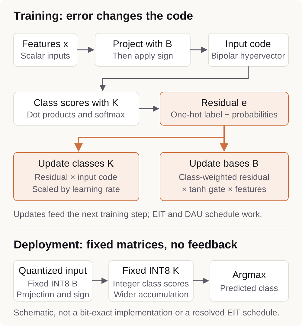
The encoder update has a familiar interpretation. The gate is the derivative of , used as a smooth surrogate around a hard sign operation. The sign function itself has no useful ordinary derivative away from its boundary. The method therefore resembles training a shallow network with a bipolar hidden representation and a surrogate backward path. Its HDC formulation makes the learning signal explicit through weighted class hypervectors and componentwise operations.
The random bases are the starting point, then. They no longer have to stay random. Labels can change the relationships among encoded samples, through updates to the bases that all samples share.
Why reuse the encoded data?
An encoder that changes throughout training cannot always reuse a dataset encoded once. TrainableHD addresses the resulting work with Encoder Interval Training (EIT). It periodically refreshes cached encoded samples, while class learning continues between refreshes. The experiments use 50 epochs, learning rate , and interval .1
EIT lets class learning continue on cached codes between refreshes. The text and Figure 3 describe the timing of base updates somewhat differently, but both show why we reuse the encoded data: we can keep learning the classes without repeating the full projection for every update.
How much work does reuse save? The authors report 89.20% less work in base updating and 69.89% less in encoding.1 Each number belongs to that part of training. We still have the other training steps to run, and we need memory to hold the cached codes.
Binary codes still need integer weights
Taking signs only binarizes the sample code. The encoder still carries floating-point bases, and so do the class weights. To use integer kernels for projection and class scoring, TrainableHD quantizes the input features as well as both weight matrices.1
Rather than round the weights only at the end, the authors simulate quantization during learning. Rounding and clipping affect the forward calculation, while floating-point values remain available for training updates. When training is finished, the matrices are converted to INT8. This is quantization-aware training (QAT).
Here’s the conversion in a conventional signed affine quantizer:
The scale stretches the floating-point range into the integer range, and the zero point supplies an offset. Rounding picks an integer; clipping keeps it between −128 and 127.2 This is the conventional affine form we use to explain the conversion. The paper expresses its quantizer in its own notation.
TrainableHD tracks moving minima and maxima with coefficient . Drift-Aware Update (DAU) postpones fake quantization until accumulated changes in the bases or classes cross a relative threshold . DAU schedules quantization simulation; EIT schedules encoder work and representation refreshes. Neither adds a learning loop to deployed inference.1
For the Xavier implementation, INT8 Tensor Core products feed an INT32 accumulator.3 The wider accumulator gives the running sum more range. We save bytes in the weights and can use integer kernels without expecting each intermediate sum to fit in eight bits.
QAT adds time to learning. On the RTX 3090, training was 24.48× faster than the paper’s deep neural network (DNN) baseline without QAT and 12.13× faster with it, averaged over the datasets. DAU cut the reported quantization overhead by 84.50%, with small reported accuracy changes from quantization and DAU.1 We get the integer model’s execution benefits after training has finished.
What improved in the experiments?
EMOTION gives the encoder 1,500 features; PAMAP2 gives it 27. Across the 12 datasets, the class counts run from 2 to 100.1 For equal hypervector widths, those input sizes change the projection cost. We’ve put Table I’s dimensions and sample counts here so we can read the results against the work each encoder has to do:
| Dataset | Training / test samples | Classes | Features |
|---|---|---|---|
| EMOTION | 1,705 / 427 | 3 | 1,500 |
| FACEA | 22,441 / 2,494 | 2 | 512 |
| FACE | 22,441 / 2,494 | 2 | 608 |
| HACT | 7,352 / 2,947 | 6 | 1,152 |
| HEART | 119,560 / 4,000 | 5 | 187 |
| ISOLET | 6,238 / 1,559 | 26 | 617 |
| MAR | 1,440 / 160 | 100 | 64 |
| MNIST | 60,000 / 10,000 | 10 | 784 |
| PAMAP2 | 16,384 / 16,384 | 5 | 27 |
| SA12 | 6,213 / 1,554 | 12 | 561 |
| TEX | 1,439 / 160 | 100 | 64 |
| UCIHAR | 7,352 / 2,947 | 6 | 561 |
The authors start with a static nonlinear encoder and retrained class hypervectors as their fixed-encoder baseline. They also compare with ManiHD, which first learns an unsupervised manifold. For the DNN, they use Ray Tune to search configurations with up to five layers, 512 neurons, and batch size 64, then train for 50 epochs.1 These are the comparators behind the accuracy and timing figures.
HACT makes the accuracy change easy to see because the paper gives the exact values:
| Dimension | Fixed-encoder baseline | TrainableHD | Difference |
|---|---|---|---|
| 3,000 | 57.28% | 78.62% | +21.34 percentage points |
| 10,000 | 59.35% | 81.61% | +22.26 percentage points |
Subtract 59.35 from 81.61 and we get 22.26 percentage points: the paper’s largest accuracy gain, on HACT at 10,000 dimensions. The averages are smaller. The authors report 3.62% at 10,000 dimensions and 2.58% at 3,000 dimensions over their fixed-encoder baseline, and 6.27% over ManiHD at 3,000 dimensions.1 Those averages retain the paper’s percentage notation. For the two HACT rows, we’ve calculated the differences directly and labelled them percentage points.
HACT is the largest gain in the suite; other datasets benefit by different amounts. Figure 7 also shows that the learned encoder can retain useful accuracy with fewer components.1 Increasing width is no longer our only option. We can also train the mapping into the components we already have.
What do we pay for training and inference?
For a dense projection and class comparisons, our operation-count model is approximately multiply-accumulate contributions per sample, plus sign and argmax. Learning does not add another inference stage at the same width. It does add encoder updates during training, along with residual computation, a surrogate gate, possible re-encoding, and fake quantization. The resulting model invests work in learning while retaining a compact deployed procedure.
The encoder can dominate both arithmetic and parameter storage when greatly exceeds . For HACT at , the dense count is 3,456,000 encoder contributions and 18,000 class-score contributions. Quantizing both the encoder and class matrix addresses the complete inference path.
Ignoring alignment, scales, buffers, and executable code, the raw parameter bytes are:
For HACT at 3,000 dimensions, those INT8 matrices occupy 3,474,000 raw bytes, about 3.47 MB. FP32 would take 13,896,000 bytes for the same matrices. Reducing the width from 10,000 to 3,000 as well as moving from FP32 to INT8 cuts raw weight storage by a theoretical factor of 13.33. This is our calculation for the matrices alone. Scales, buffers, alignment, and training intermediates still need space; the calculation isn’t a measured device footprint.
A cache of bipolar samples needs bytes if bit-packed, if held in INT8, or if held in FP32. For HACT’s 7,352 training samples and , the packed minimum is 2,757,000 bytes. Training storage also includes any pre-sign values and other intermediates that the implementation retains.
Putting the classifier on hardware
Getting this classifier onto hardware takes more than converting the weights. For x86, the authors adapt FBGEMM to handle integer operations and sign. On Jetson Xavier they use cuBLAS and Tensor Cores; on a Xilinx Zynq-7000 FPGA they build a systolic implementation based on lookup tables. They also arrange or buffer parameters for reuse.1 These implementation choices help turn the arithmetic into the reported hardware results.
Here are the timing and energy figures, with each device’s comparator. Training and inference have separate rows:
| Phase and implementation | Reported comparison | Scope |
|---|---|---|
| RTX 3090 training, without QAT | 24.48× average speedup over DNN | Training on this GPU |
| RTX 3090 training, with QAT | 12.13× average speedup over DNN | Includes quantization simulation |
| Xavier GPU inference, FP32 | 56.4× faster, 73× better energy efficiency | Versus DNN inference on Xavier |
| Xavier GPU inference, INT8 | Additional 3.1× speed improvement | Over TrainableHD without quantization |
| Xeon Silver 4110 inference, INT8 | 20.7× faster | Versus the GPU DNN baseline |
| Zynq-7000 FPGA inference, INT8 | 180.8× faster, 167.8× better energy efficiency | Versus the GPU DNN baseline |
Start with the Xavier FP32 row. The 56.4× speedup and 73× energy-efficiency improvement are already present before INT8 conversion; quantization then adds a further speed improvement. For the CPU and FPGA rows, follow the comparator column: both use the GPU DNN as the reference.1 Device choice is part of those comparisons.
The measurements use Intel RAPL, NVIDIA Nsight, and the Xilinx Vitis toolkit. To estimate performance for our own workload, we’d also need its batch size, preprocessing, and device settings. Xavier alone has several power modes.3 These results give us a useful starting point for deployment, with the hardware and workload kept beside the numbers.
Where TrainableHD fits
NeuralHD had already taken encoder learning into HDC in 2021. It selects dimensions for regeneration using statistics of the class hypervectors.4 TrainableHD’s base-learning rule works through the classification error instead: weight the classes by their residuals, apply the gate, and move the dense bases. Both let training alter the representation, through different update mechanisms.
We can place the other earlier methods by following what they learn. ManiHD learns an unsupervised manifold projection, which can be folded into the HD projection for deployment.5 LeHDC trains the class hypervectors and keeps its encoder fixed.6 LDC goes further into the representation, learning value, feature, and class representations together.7
QuantHD had explored quantizing class models, while QAT was already used to prepare neural networks for integer inference.82 In TrainableHD, we get supervised learning of the bases and classes, a schedule for reusing encoded data, and a path to INT8 execution in one system.
HDC Labs discussion: following one incident through training
Imagine an incident desk deciding which reports need escalation. We’ll give it just two features: did the incident happen overnight, and did it cause customer data loss? Let’s follow a daytime incident with data loss through one training step. We made up the numbers for this HDC Labs discussion. This isn’t an experiment from the paper, and our four-component hypervectors are small enough to inspect by eye.
A fixed encoder would already let us learn class memories by adding labelled incident codes, then retrain those memories after mistakes. TrainableHD also lets us change the bases used to encode future incidents. Our example follows that extra update.
Encode a daytime incident with data loss
Suppose we’re partway through training and the data-loss base has the components below. Our incident happened during the day and caused data loss, so the inputs are zero for overnight and one for data loss:
overnight = 0
data_loss = 1
h_base,data_loss = [0.2, 0.2, -0.2, -0.2]

h_pre   = 0 × h_base,overnight + 1 × h_base,data_loss
        = [0.2, 0.2, -0.2, -0.2]
h_input = sign(h_pre) = [+1, +1, -1, -1]
Here, one just multiplies the data-loss base. We aren’t creating a separate hypervector for the value one, or binding a role hypervector to a value hypervector. The encoded incident is the sum of its scaled feature bases.
Compare the code and form the residual
Now suppose the current class hypervectors point in opposite directions:
h_class,routine    = [+1, +1, -1, -1]
h_class,escalation = [-1, -1, +1, +1]

Routine score:    +4
Escalation score: -4
The classifier confidently calls this incident routine, but the label says it needs escalation. Softmax gives routine a probability of about 0.9997 and escalation about 0.0003. In the order routine, escalation, the target is [0, 1], so the residual is approximately [-0.9997, +0.9997]. The signs tell us which class has received too much probability and which has received too little.
Update the classes and the shared bases
First, the class update subtracts a small multiple of the incident’s code from the routine class and adds it to the escalation class. Next, the base update uses the residual-weighted classes, the gate, and the input features. With learning rate 0.01 and Algorithm 1’s class-first order, the data-loss base becomes approximately:
h_base,data_loss = [0.1810, 0.1810, -0.1810, -0.1810]Look at the signs: they’re still positive, positive, negative, negative. Both halves of the data-loss base have moved toward zero, but no component has crossed it. We therefore get the same bipolar code and the same routine prediction, although the class-score margin is narrower. The overnight base hasn’t moved, since its input was zero. A single step has changed the continuous weights before changing the decision.
The updated data-loss base now sits in the shared encoder, ready for the next incident. An arriving incident uses the base as it stands; it doesn’t repeat the previous training correction. If we supply numerical features, their values scale the bases before summation. The signs come from that combined sum.
This is the connection we wanted to make with semantic compression inside wide hypervectors.9 The classes learn how to compare the codes; the encoder learns how to produce codes useful for that comparison. We haven’t added more components. We’ve changed the mapping from features into them. The adjustment is distributed across the bases, so it doesn’t give us a single readable importance coefficient for each feature.
Keep the 2023 result in its time
A TrainableHD journal article followed in ACM Transactions on Design Automation of Electronic Systems in 2024. Its institutional record describes further work on adaptive training and optimizers.10 Here, we’ve stayed with the methods and results of the DATE 2023 paper.
This paper gives us a useful option when a fixed encoder needs more dimensions than we want to deploy. We could learn the bases as well as the classes, then use EIT and DAU to manage the training work and quantization to prepare the integer model. The experiments show what that combination achieved in 2023.
Our incident still needs escalation, and one update hasn’t taught the classifier to recognize it. By carrying the feedback into the shared bases, we’ve given later training steps a way to change how incidents are represented, so learning can improve the hypervectors that future decisions depend on.
References
Footnotes
-
Jiseung Kim, Hyunsei Lee, Mohsen Imani, and Yeseong Kim. Efficient Hyperdimensional Learning with Trainable, Quantizable, and Holistic Data Representation. DATE 2023. Proceedings PDF. DOI: 10.23919/DATE56975.2023.10137134. Reviewed in full, including all figures and the bibliography. Method: Sections III to V, Algorithm 1; evaluation: Table I and Figures 5 to 11. ↩ ↩2 ↩3 ↩4 ↩5 ↩6 ↩7 ↩8 ↩9 ↩10 ↩11 ↩12 ↩13 ↩14
-
Benoit Jacob and colleagues. Quantization and Training of Neural Networks for Efficient Integer-Arithmetic-Only Inference. CVPR 2018. Author manuscript, conference PDF. Sections 2 and 3 explain affine quantization, accumulators, and simulated quantization during training. ↩ ↩2
-
Dustin Franklin. NVIDIA Jetson AGX Xavier Delivers 32 TeraOps for New Era of AI in Robotics. NVIDIA, 2018. Hardware description. Tensor Core and power-mode descriptions provide hardware context, not independent verification of TrainableHD’s measurements. ↩ ↩2
-
Zhuowen Zou, Yeseong Kim, Farhad Imani, Haleh Alimohamadi, Rosario Cammarota, and Mohsen Imani. Scalable Edge-Based Hyperdimensional Learning System with Brain-Like Neural Adaptation. SC 2021. Paper PDF, DOI: 10.1145/3458817.3480958. Sections 3.1 and 3.3 describe dynamic dimension regeneration. ↩
-
Zhuowen Zou, Yeseong Kim, M. Hassan Najafi, and Mohsen Imani. ManiHD: Efficient Hyper-Dimensional Learning Using Manifold Trainable Encoder. DATE 2021. Author-hosted PDF. Sections III-B and IV-A describe the learned manifold, projection folding, and online updates. ↩
-
Shijin Duan, Yejia Liu, Shaolei Ren, and Xiaolin Xu. LeHDC: Learning-Based Hyperdimensional Computing Classifier. DAC 2022. Author manuscript, arXiv v2, DOI: 10.1145/3489517.3530593. Sections 3 and 4 distinguish learned class hypervectors from the unchanged encoder. ↩
-
Shijin Duan, Xiaolin Xu, and Shaolei Ren. A Brain-Inspired Low-Dimensional Computing Classifier for Inference on Tiny Devices. tinyML Research Symposium 2022. Author manuscript, arXiv v2. Section 3 describes end-to-end learning and extraction of value, feature, and class representations. ↩
-
Mohsen Imani and colleagues. QuantHD: A Quantization Framework for Hyperdimensional Computing. IEEE TCAD, published online in 2019. Public author manuscript, DOI: 10.1109/TCAD.2019.2954472. Section III describes binary and ternary model quantization with retraining. ↩
-
David Hughes and Prashanth Rao. Semantic compression inside wide hypervectors. HDC Labs, 2026. Public article. Later conceptual context for the HDC Labs teaching discussion. ↩
-
Jiseung Kim, Hyunsei Lee, Mohsen Imani, and Yeseong Kim. Advancing Hyperdimensional Computing Based on Trainable Encoding and Adaptive Training for Efficient and Accurate Learning. ACM TODAES 29(5), 2024. Institutional record and abstract, DOI: 10.1145/3665891. Institutional metadata and abstract reviewed. ↩