
Connecting the dots in hyperspace: Why we built lance-csr
We introduce lance-csr, a fast graph query engine over Lance datasets that enables exact queries in Cypher or SQL, and associative search with hypervectors over a single copy of the data.


On this page
The most important questions rarely begin with an exact name or ID. So often, we only have partial information. We may have enough to recognize a plausible match, but perhaps not enough to write a query that requires every detail to be correct. How do we search with the knowledge we have, and then follow the connections that help us make sense of the answer and evolve our hypothesis?
From an HDC perspective, connected data offers two complementary views of the same situation: explicit connections to follow, and graph-like patterns we can model in hyperspace. Putting these ideas to work raises practical questions, especially when you realize real-world data is typically multimodal (i.e., a mix of structured records, images, learned embeddings, and hypervectors).
At HDC Labs, we tend to store multimodal data in Lance, an open-source, columnar, multimodal lakehouse format that supports these use cases well. Associative search over these records depends on graph queries at two points, and both often span several hops (requiring joins).
Before we can search, we need to gather the connected facts around each record and encode them as hypervectors. Once a hypervector search surfaces plausible candidates, we need to follow their exact relationships to inspect them. Ideally, we’d do both over the same records, without copying them into a separate graph database and keeping another system in sync.
To solve these problems, we need a capable graph query engine that sits close to our data. This is what led us to build lance-csr, a fast graph query engine over Lance datasets. It runs embedded (no servers), inside an application, on a single machine, directly over existing Lance datasets. It provides the exact graph-query capabilities we (and many other graph developers) need.
Explore lance-csr on GitHub An open-source graph query engine over Lance, built in Rust 🦀 on Apache DataFusion.For our HDC needs, we’ll next look at why we want graph queries alongside Lance’s indexing and vector search capabilities over the same underlying connected data.
Why we forked lance-graph
There was already a Cypher-capable query engine on top of Lance called lance-graph. However, the project fell dormant, and it lacked support for several openCypher constructs. Still, lance-graph contained a well-designed Cypher parser and schema builder, and already used Apache DataFusion for its query planning.
DataFusion is a modular, embeddable query engine written in Rust, with a mature ecosystem around it. Its built-in operators already handle the work every data system needs, such as filtering, joining, sorting, and aggregating rows. Developers can then focus on what’s specific to their application and add it as custom operators. For us, that meant reusing DataFusion’s standard operators and building only the graph-specific ones for following relationships.
So we forked lance-graph and rewrote its internals as lance-csr, keeping DataFusion as the engine underneath. To begin, we added a compressed sparse row (CSR) index (more on this below) that makes it efficient to follow relationships, and we also broadened the subset of openCypher that lance-graph supports, to be able to run a much more comprehensive set of queries.
The latest versions of lance-csr run an adapted suite of all 14 SNB Interactive complex read queries1 from the Graph Data Council (GDC). Along the way, we also added several other features, including OPTIONAL MATCH, chained WITH clauses, list comprehensions, and shortestPath algorithms that are common in other graph systems.
Let’s see how lance-csr works in practice, using a small synthetic dataset to illustrate the key ideas.
Example app: Find someone at Maker Night
Maker Night is a fictional community of 26 people who form 44 friendships. Their interests include photography, robotics, music, and gardening. Friends tend to gather in social groups around these interests, with some friendships connecting different groups. The group names in the diagram help us follow the example, and the queries below use each person’s own interests and the friendships between them.
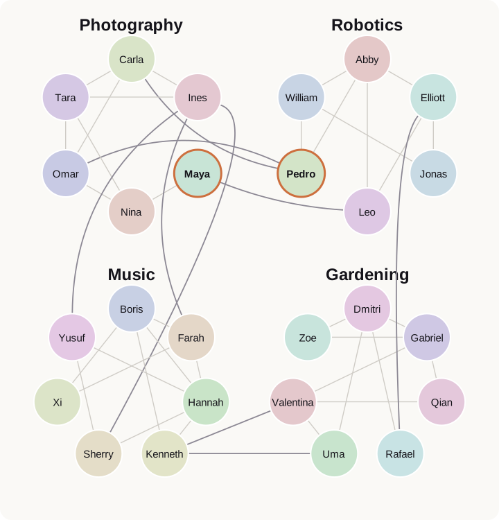
All the data lives in two Lance tables. A Person node table holds names, attributes, interests, and synthetic portraits (bytes) of each person. A FRIEND_OF relationship table holds one row per friendship, identified by its two person IDs. Any derived embeddings and hypervectors associated with a person are additional columns of the Person table.
You can rebuild these tables and rerun every query and search in this post with the lance-csr-demo code on GitHub.
Maya can only remember partial information to begin with: a man interested in robotics, with black hair, who also knew someone in the photography group. (So often the case in reality!) Maya wants to find Pedro, but she doesn’t yet know his name. Also, her recollection might be wrong about a detail.
Depending on how sure Maya is, we can ask her question of the graph in two ways:
| What Maya can provide | What she needs back |
|---|---|
| Exact facts about the man and his friend | People whose graph neighbourhood satisfies every condition |
| A few remembered cues, possibly mistaken | People whose graph neighbourhood resembles those cues |
Start with an exact graph pattern
Let’s start by turning what Maya remembers into a graph query. She’s looking for a man with black hair who’s interested in robotics, and she remembers that he knows someone who does photography. The hair and robotics clues describe the man himself. Photography describes a friend, so we need to follow a friendship edge before checking that interest.
In Cypher, we can match the personal clues first, then add a second MATCH to follow the friendship:
MATCH (p:Person)
WHERE p.gender = 'male' AND p.hair_colour = 'Black'
  AND 'robotics' IN p.interests
MATCH (p)-[:FRIEND_OF]-(f:Person)
WHERE 'photography' IN f.interests
RETURN DISTINCT p.name AS name
ORDER BY name
The second MATCH reuses the candidate p from the first clause and follows a FRIEND_OF edge to f. We filter on “photography” in the friend’s interests, just as we filtered on “robotics” in the candidate’s interests. The assumption is that the friendship relationship connects the two individuals across these groups. The DISTINCT keyword in Cypher keeps one result per person even when several friends fit the pattern.
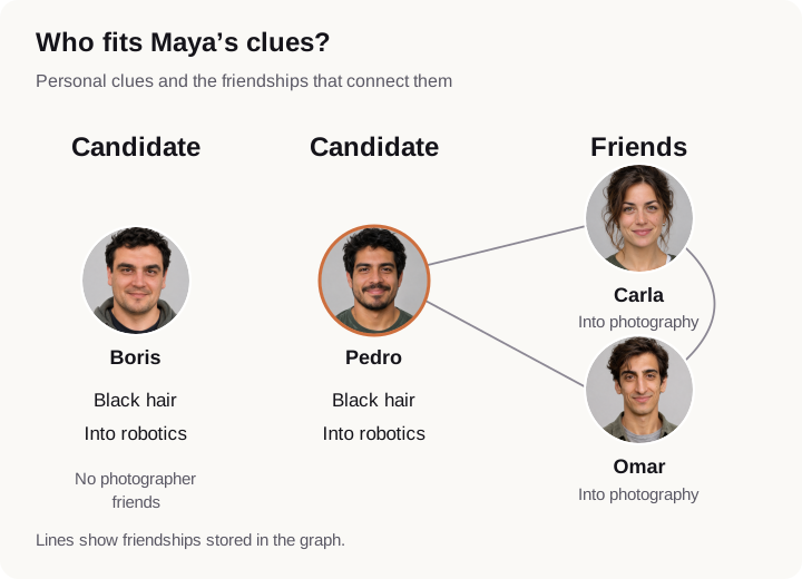
Per our results, Pedro has black hair, is interested in robotics, and is friends with Carla and Omar, who are both interested in photography. Boris also fits the personal clues, but none of his friends has photography listed as an interest. In this dataset, only Pedro satisfies the full query, and is the person Maya is looking for.
Now, imagine that the query changes just the hair colour filter from “black” to “dark”, because Maya only remembers that her person of interest had “dark hair”. However, “dark” is not a property value that exists in the stored data. Our exact match approach in Cypher would return no results. Ideally, we’d want both black- and brown-haired candidates to surface.
This is the intuition behind associative search: something we remember can help us recall the broader situation it’s associated with. Maya may remember “the robotics person who knew a photographer” before she remembers his name. By encoding properties and relationships together as hypervectors, we can use that association to search for connected patterns, including paths, rather than only similar individual nodes.
lance-csr doesn’t perform associative search by itself, but it augments it with fast graph traversal. It gathers the connected facts we encode as hypervectors, and once the search surfaces plausible candidates, it follows their exact relationships.
How lance-csr follows relationships
lance-csr reads the graph directly from existing Lance tables, without exporting the records to another graph database. A graph configuration builder maps those tables to node labels and relationship types. Each FRIEND_OF row holds one friendship, with src_id and dst_id pointing to the two people in Person:
from lance_csr import CypherEngine, GraphConfig

# Map node and relationship tables to their respective
# labels that we want to query in Cypher.
graph = (
    GraphConfig.builder()
    .node_table("Person", "person_id")
    .rel_table("FRIEND_OF", "Person", "Person", "src_id", "dst_id")
    .build()
)
# CypherEngine runs Cypher queries over the mapped Lance datasets
# use_csr=True builds the CSR index in memory.
engine = CypherEngine(graph, datasets, use_csr=True)
What is a CSR index?
To traverse a path stored in relational tables, a SQL or Cypher query can use joins to match rows across those tables. To follow one friendship from Pedro, the first join matches his ID in Person to a row in FRIEND_OF, and the second uses the ID at the other end of that friendship to find his friend in Person. Each additional hop repeats those two joins. One way to match the rows is a hash join. The engine builds a hash table from one input, keyed by person ID, then looks up IDs from the other input to find the matching rows.
A CSR (compressed sparse row) index stores each node’s neighbour IDs contiguously, with offsets marking where its list begins and ends. Most node pairs in the graph aren’t connected, so the equivalent adjacency matrix is “sparse”. The CSR stores only the connections, omitting the matrix’s zeros. Two offset lookups locate the start and end of a node’s neighbour list in constant time. The engine then follows the IDs stored there, reusing the CSR index instead of building a hash table for each query.
To check whether Pedro knows someone interested in photography, we first need to find his friends. The CSR index, built from the relationship table’s endpoint IDs, lets us locate those friends directly using the two offsets shown below:
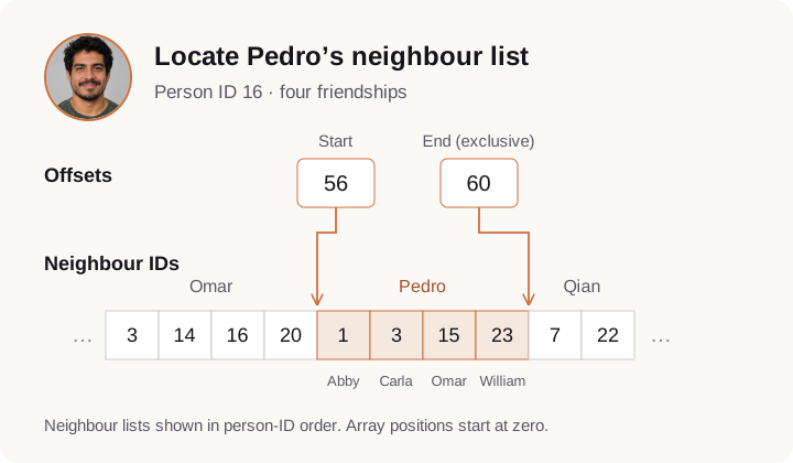
Looking up Pedro’s slice gives Abby, Carla, Omar, and William. We can follow these friendships without scanning the relationship table again. Node properties, such as each friend’s name or interests, are fetched from Person as needed. The 44 stored friendships yield 88 adjacency entries for traversal in either direction.
We pay a one-time upfront cost of organizing the friendships when we build the CSR, but we can then reuse those neighbour lists across queries. The tradeoff is that we need extra memory for the CSR index, while the underlying records stay in Lance.2 A plain SQL join needs no such setup, but if you intend to run fast multi-hop queries, the upfront work and added memory costs are worth it.
Parse the query to build an executable plan
lance-csr accepts SQL queries over the same data. Cypher passes through our graph mapping, while SQL enters through DataFusion’s SQL planner. Both routes converge on DataFusion’s execution framework, so equivalent filters, projections, and joins can compile to the same physical operators.
A query moves through these plans from top to bottom: Cypher starts with a graph plan, while SQL starts directly at the DataFusion logical plan.
| Plan | What it describes | Where it lives |
|---|---|---|
| Graph plan | Graph operations, such as finding a person and expanding to their friends. | In lance-csr, before translation into DataFusion. |
| DataFusion logical plan | Scans, filters, projections, joins, and graph expansions. | Within DataFusion, using its standard plan nodes alongside lance-csr extensions such as CsrExpand. |
| DataFusion physical plan | The executable operators that carry out those steps. | Within DataFusion’s execution framework, combining standard operators with custom implementations such as CsrExpandExec. |
An operator represents one step in a query plan, such as scanning a table, filtering rows, or joining two inputs. DataFusion lets us extend these plans with our own operators. When lance-csr translates a friendship traversal into a DataFusion logical plan, it can insert a custom logical operator CsrExpand, which describes expanding the input nodes to their neighbours using the CSR index.
To make that step executable, lance-csr registers an extension with DataFusion’s physical planner. The extension translates CsrExpand into CsrExpandExec, our implementation of DataFusion’s execution interface. It receives Arrow record batches containing node IDs, reads their neighbour lists, and produces record batches for the next operator. In Maya’s query, this is the step that takes us from a candidate person to their friends.
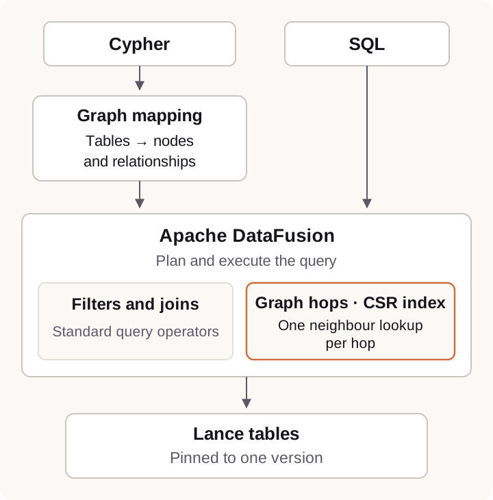
From a user perspective, lance-csr lets you use familiar SQL for tabular questions and Cypher for connected patterns, with CSR operators handling supported graph traversals. Choosing a query language doesn’t require moving the data or switching execution engines.
Why several hops change the plan
We’ll show a plan breakdown for a multi-hop path traversal between Maya and Pedro to contrast how traditional hash joins and CSR handle multi-hop traversals. To begin, let’s use the shortestPath function to find the shortest path length between these two people:
MATCH path = shortestPath(
  (m:Person {name: 'Maya'})-[:FRIEND_OF*1..10]-(p:Person {name: 'Pedro'})
)
RETURN length(path) AS introductions
The shortest path between Maya and Pedro has three hops. We’ll use the following fixed 3-hop query to compare the hash-join and CSR plans:
MATCH (m:Person {name: 'Maya'})-[:FRIEND_OF]-(a:Person)
      -[:FRIEND_OF]-(b:Person)
      -[:FRIEND_OF]-(p:Person {name: 'Pedro'})
RETURN a.name AS ask_first, b.name AS who_knows_pedro
ORDER BY ask_first
With the CSR enabled or disabled (i.e., using the traditional hash join that DataFusion picks by default), the query returns the same results, but the CSR produces a very different execution plan. Let’s compare them, reading the figure below from bottom to top:3
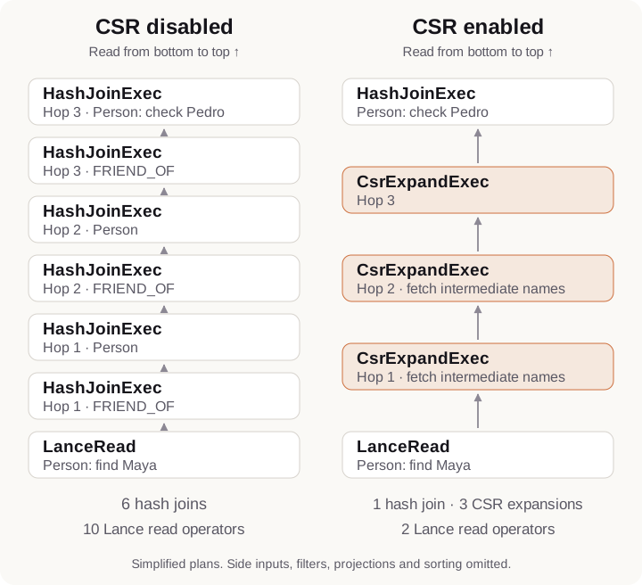
Both plans begin by finding Maya. On the left (without the CSR), each hop runs a hash join on the FRIEND_OF table to find the connections, and then another hash join to Person to find the people. On the right, CsrExpandExec reads the prebuilt neighbour lists and fetches the intermediate names, leaving one hash join to check that the path ends at Pedro. In this 3-hop query, the CSR turns six hash joins into a single hash join, which is a substantial reduction in work.
Search the graph with partial cues in hyperspace
Let’s return to Maya’s original search, to understand how lance-csr works well alongside associative search. As Maya recalls details one at a time, we’d like our retriever to surface plausible candidates, which is simple because we’re essentially doing top-k vector search over the stored hypervectors.
From the initial query, we encode each person’s attributes together with facts about their friends and people farther away, using the approach we described in our earlier post. Once the hypervectors are stored, we can search them with Maya’s first clues and add others as she remembers them.
Start with black hair
Maya is sure she saw a man, but less sure about his hair: was it black or dark brown? We can use gender = 'male' as an exact filter and put the uncertain hair clue in the hypervector. Binding () pairs the hair attribute with the value Black to form a hypervector for the first cue:
We compare this query with the candidates’ stored hypervectors using cosine similarity. Here are the top 3 results:
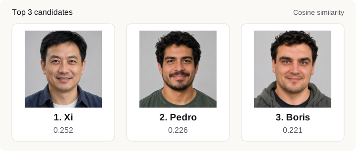
Maya now has faces to consider, but black hair alone gives her little to go on.
Add an interest in robotics
Next, she remembers that the man was also interested in robotics. Let’s bundle () that cue with the hair cue and search again:
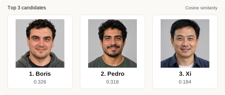
Boris and Pedro now lead with similar scores. Both have black hair and an interest in robotics, just as we saw in the exact graph query.
Add a friend who does photography
Next, say Maya remembers that the man knew someone who shared her interest in photography. We used a friendship edge to express this clue in the second Cypher MATCH. How can we express the same one-hop relationship in the hypervector query?
We bind photography to the same interest attribute we used for robotics. Because photography describes a friend rather than the candidate, we apply a permutation operation () once to mark that fact as one hop away:4
The equation above is the HDC way of expressing this kind of path:
Black hair and robotics describe , on the left. Photography describes , one hop away in the graph. The friendship edge in Cypher and the permutation in HDC both distinguish a candidate’s own interest from a friend’s interest. Without the permutation, bundling robotics and photography would lose which interest belonged at which hop.
We apply the same permutation when encoding the stored neighbourhoods and when building the query. These representations use people’s attributes, interests, and facts reached through friendship paths; they don’t include a community label. Running the query gives us the following ranked shortlist:
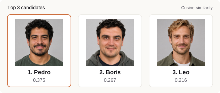
Pedro, the right person, now leads the shortlist. His own interest in robotics and his friends Carla and Omar’s interest in photography contribute to the match. Pedro also likes photography himself, but the permuted cue asks about his friends’ interests.
We can also compare the two searches when Maya gets the hair colour wrong, keeping robotics and the photographer-friend clue fixed:
| Hair cue | Exact Cypher result | Hypervector shortlist, in rank order |
|---|---|---|
| Black | Pedro | Pedro, Boris, Leo |
| Dark brown | William | William, Elliott, Pedro |
With the mistaken cue, Pedro drops to third in the ranked search rather than disappearing. Maya can still inspect his friendships and decide whether she misremembered his hair. We built up the same personal facts and one-hop relationship in both searches, but used them differently: Cypher required every condition to hold, while each hypervector cue contributed to similarity.
The bundled hypervector retains which hop a fact came from, but it is a lossy summary of the neighbourhood. It does not preserve the full topology or keep every friend’s attributes grouped together. The explicit graph remains available to check the exact relationships behind a proposed match.
Conclusions
We built lance-csr to make it practical to combine fast associative search and graph traversal over Lance. Graph queries (expressed in Cypher or SQL, whichever is easier) let us gather the connected facts, hypervectors make those associations searchable, and exact traversals let us inspect the results. The graph and its high-dimensional representations share the same underlying records, giving us more ways to ask questions as our understanding develops.
lance-csr is also a general-purpose graph query engine, which we will continue to maintain at HDC Labs. We see a future where lance-csr can be used in applications that need multi-hop graph queries over Lance, whether or not they use hypervectors. lance-csr is regularly benchmarked against the GDC SNB SF1 dataset over complex query patterns, so any performance improvements that DataFusion and Lance themselves provide directly benefit lance-csr too.
We’d love to work with the open-source community to help push multi-hop graph traversal performance further on top of the already mature DataFusion and Rust 🦀 ecosystems. There’s always room for better query plans, specialized operators, and new benchmarks across varied workloads. If you’d like to contribute or build on top of it, explore the project below and see the contribution guide. And if you want to know more about what we’re building, get in touch. We’d love to hear from users! 🚀
Explore lance-csr on GitHub An open-source graph query engine over Lance, built in Rust 🦀 on Apache DataFusion.Footnotes
-
We use the GDC (formerly the Linked Data Benchmark Council, or LDBC) Social Network Benchmark dataset and workloads for benchmarking. Our custom Python-based complex-query harness uses the GDC SF1 dataset and adapts the 14 complex read queries from the SNB Interactive v1 reference implementations. These are independent, unaudited runs, not official GDC/LDBC Benchmark Results. Maker Night is our separate synthetic teaching dataset only for this post. ↩
-
Specialized graph systems like Kùzu and its fork LadybugDB integrate disk-backed CSR storage into native relationship tables, loading pages into memory as needed. Lance has no native relationship-table primitive, so lance-csr builds a separate adjacency index over ordinary tables. It can save that index to avoid rebuilding it at startup, but currently loads the whole CSR into memory for traversal. Future versions may read adjacency from disk as needed, reducing the amount of the index that must remain in memory. ↩
-
lance-csr provides an
engine.explain(query)convenience method, wherequeryis the Cypher string. This lets you inspect the graph, logical, and physical plans the engine generates without executing the query. You can compare engines created withuse_csr=Falseanduse_csr=Trueto see how the same query is planned with and without the CSR index. ↩ -
A permutation rearranges a hypervector’s coordinates in a fixed order. We apply it once for one-hop facts, twice for two-hop facts, and so on, using the same transformation in the stored representation and query. ↩