Semantic compression inside wide hypervectors

A useful representation leaves things out. It keeps distinctions that help a system recognize, compare, or act, while letting other details disappear. But HDC often takes an already compact representation and expands it into thousands of coordinates. Why spend so much space carrying something we’ve worked to simplify?

The apparent contradiction comes from counting two different things: the distinctions a representation preserves and the width of the code that carries them. A representation can be semantically compressed while its code is computationally expansive. Here, semantic compression means discarding distinctions judged irrelevant to a task; it doesn’t imply a particular compression algorithm or a measured information-theoretic optimum.

Barrett and Miller describe how the brain compresses sensory detail into summaries useful for action, while feedback shapes how new signals are processed.¹ Their account points us to two choices in an HDC pipeline: which differences should the encoder keep, and what do we gain by spreading the remaining features across a wide hypervector? We’ll follow the information through both steps, then ask when more width helps us compare, combine, and retrieve representations, and when we need to revisit what the encoder kept.

Count the distinctions, then count the coordinates

Imagine an image encoder trained to recognize an object across changes in lighting. Ideally, its output retains the differences needed for recognition while becoming less sensitive to illumination. Mapping that output into 10,000 coordinates needn’t bring the discarded lighting detail back. More coordinates can describe the same retained distinctions in another form.

We need a few separate quantities to explain why:

Quantity	What we’re counting
Ambient dimensionality	The coordinate axes in the surrounding mathematical space.
Representation width	The number of components actually used by a code. For a dense hypervector in $\mathbb{R}^{D}$, this is $D$.
Intrinsic dimensionality	The degrees of freedom needed to describe the data’s variation under a specified geometric model and scale.
Information content	Uncertainty or distinguishable states under an explicit probability and precision model. Coordinate count alone doesn’t determine it.
Distributed coding	How information is spread across components, rather than assigned to one dedicated component per concept.

Intrinsic dimensionality isn’t automatically a count of human-readable semantic features. A low-dimensional representation can retain nuisance variation, and useful abstractions needn’t have neatly separable coordinates. Likewise, a cortical dimensionality estimate and an HDC component count measure different objects.

Kanerva makes the underlying engineering distinction in his foundational HDC tutorial: the dimensionality of what is represented and the dimensionality chosen for computation are separate questions.² Our compression argument applies that distinction to a pipeline with learned features.

Expansion doesn’t undo abstraction

Take two photos of the same object, one in bright light and one in shade. An encoder trained for recognition may keep features common to both while becoming less sensitive to lighting. HDC can spread those features across 10,000 components, but spreading them doesn’t change what the encoder kept. Any lighting information still present is carried along; details it discarded stay lost.

Let’s view how this works with symbols. Let $x$ be a photo and $z=f(x)$ its feature vector with $d$ coordinates. A fixed projection $R$ maps it to a real-valued hypervector $\mathbf{h}_{x}$ with $D$ components:

$$z\in\mathbb{R}^{d},\qquad R\in\mathbb{R}^{D\times d},\qquad \mathbf{h}_{x}=Rz,\qquad D>d.$$

Each output component mixes the features in $z$. The first step in the figure below is abstraction: for object recognition, the encoder can treat a bright and a dim photo as similar despite their different pixel values. The second step is also encoding; we call it recoding because the projection takes features the image encoder already produced and spreads them across a wider hypervector. Because the projection sees only $z$, it cannot recover a difference the encoder removed. Two photos that produce the same $z$ therefore produce the same $\mathbf{h}_{x}$.

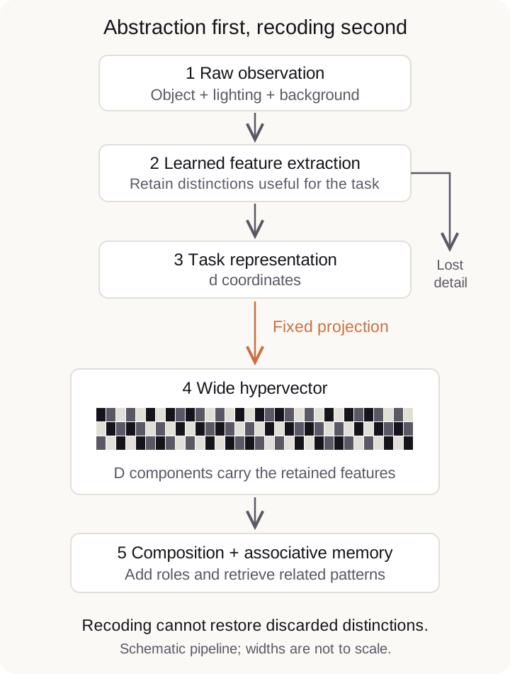
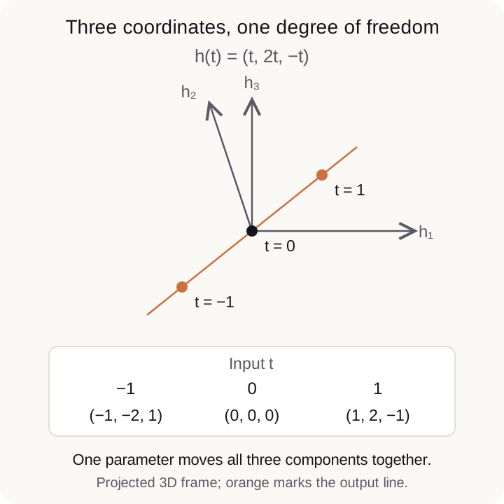
Linear expansion also doesn’t create $D$ independent degrees of freedom. Every output lies in the column space of $R$, whose dimension is at most $d$. Projecting 64 input coordinates into 10,000 output coordinates therefore allows at most 64 independent directions of variation. The next figure illustrates this limit with one input coordinate mapped to three output coordinates.

Some encoders then quantize the output, for example with $\mathbf{h}_{x}=\operatorname{sign}(Rz)$. The linear subspace argument no longer describes these bipolar codes, but identical feature vectors still produce identical codes. Quantization may discard more detail; it cannot restore what the encoder removed.

Expanding the code cannot repair an abstraction that erased a needed distinction. If two objects the task must tell apart already have identical feature vectors, increasing width will give both the same hypervector. To fix this, we need to change what the encoder keeps. Once the needed distinctions survive, we can ask whether extra width makes comparison, composition, or retrieval more reliable.

What the width can buy

Kanerva describes distributed patterns, associative cleanup, and composition through operations on representations of a common width.² Whether those operations justify recoding the features depends on the task.

One benefit can be more stable similarity estimates. Consider a sign encoder whose matrix rows are sampled independently from an isotropic Gaussian distribution, then fixed and shared across inputs. For two nonzero inputs separated by angle $\theta$, the probability that a coordinate disagrees is $p=\theta/\pi$.³ Across $D$ independent rows, the mismatch fraction estimates that probability:

$$\mathbb{E}[\widehat p]=p,\qquad \operatorname{SD}(\widehat p)=\sqrt{\frac{p(1-p)}{D}}.$$

Increasing width reduces the sampling variation in this estimate across random encoders. It doesn’t improve the semantics of the original features, guarantee every nearest-neighbor ranking, or preserve numerical cosine similarity unchanged. The expected bipolar cosine is $1-2\theta/\pi$. The exact angular result relies on isotropic directions; it isn’t a universal formula for arbitrary projection matrices.

HDC also gives the encoded features a common format in which to compose associations. For example, a task description can bind an object and a goal to distinct roles, then bundle the pairs:

$$\mathbf{h}_{\text{description}} = (\mathbf{h}_{\text{object-role}}\otimes\mathbf{h}_{\text{object}}) \oplus (\mathbf{h}_{\text{goal-role}}\otimes\mathbf{h}_{\text{goal}}).$$

Here the role hypervectors identify the two fields, and the value hypervectors carry the object and goal. The result remains $D$ components wide. The goal supplies additional information explicitly; widening the object representation alone would not create it.

Possible benefit	Condition we still need to check
Separation of unrelated patterns	Independent random codes tend toward near-orthogonality; correlated learned inputs needn’t.
Tolerance of component corruption	Retrieval needs enough remaining evidence and a sufficient margin from competing memories.
More room for superposition	Recovery depends on width, bundle size, correlations, precision, and the cleanup memory.
Simple componentwise operations	Total cost still includes encoding, storage, comparisons, and data movement.

These are reasons to evaluate a wide representation, not a promise that wider is always better. Similarity error may shrink while application accuracy stays flat. A larger code can also cost more to construct and search than the original features.

Choose width around the work

Our earlier post on where meaning in a hypervector comes from explored projecting learned features into HDC. The HDC Labs question here is what the additional width earns once those features enter a memory system. We would compare widths while keeping the feature extractor and evaluation task fixed.

Measurement	What it would tell us
Neighborhood preservation and retrieval accuracy	Whether recoding keeps the relationships the application needs.
Retrieval under controlled code corruption	Whether distributed redundancy helps with the specified failure model.
Recovery as bundle size grows	How composition changes interference and cleanup success.
Storage, encoding cost, and query latency	Whether the benefit survives the full pipeline’s costs.

This is a proposed comparison, not a reported experiment. It needs a direct feature-space baseline, several random seeds, and separate tests for noise before encoding and damage after encoding. Those two disturbances ask different questions. If direct feature retrieval meets the requirements more cheaply and composition adds no value, expansion may be unnecessary.

The practical principle is to preserve the distinctions the task needs, then choose a representation that makes the required operations reliable and affordable. A wide hypervector can serve a compact abstraction without reversing it. The next question is how the system changes which distinctions matter when its context changes. Our next post will examine how context can influence retrieval itself.

Footnotes

1. Lisa Feldman Barrett and Earl K. Miller, “Categorization is ‘baked’ into the brain” ↗ , Nature Reviews Neuroscience (2026). Open author PDF ↗ . This Perspective motivates the series; the HDC constructions here are our engineering analysis. ↩

2. Pentti Kanerva, “Hyperdimensional Computing: An Introduction to Computing in Distributed Representation with High-Dimensional Random Vectors” ↗ , Cognitive Computation 1 (2009): 139-159. Open author manuscript ↗ , especially sections 3.1, 4.2-4.3, and 6.1-6.9. ↩ ↩²

3. Moses S. Charikar, “Similarity Estimation Techniques from Rounding Algorithms” ↗ , STOC 2002: 380-388. Open paper ↗ , section 3. The variance expression above follows from averaging independent Bernoulli disagreement indicators. ↩