Testing the limits of bundling capacity (2)

In part 1 of this series, we looked inside a bundle: as we packed more facts into one hypervector, how much could we recover? There, the limit came from crosstalk between facts within a single record, so it depended only on how we encoded. This time, we look across many bundles and ask: how many records can a 2,048-dimensional hyperspace hold before unrelated records start to look alike?

Here, unrelated records have no encoded facts in common: none of their property values match. Any similarity between their hypervectors is therefore accidental.

To decide whether a hyperspace is “big enough”, we need to know its dimension and how many comparisons we make. The dimension sets the chance that two unrelated records produce a false positive. The application sets how often we take that chance. Even a tiny probability adds up when we compare enough records.

Imagine a social network app that suggests contacts based on what people have in common, such as an employer or an interest. When the user Maya opens the app, it compares her hypervector with everyone else’s and asks: does anyone unrelated look like Maya? If the app also groups people into communities, it needs to compare everyone with everyone else, so our question becomes: do any two unrelated people look alike? The second question makes vastly more comparisons, so as the dataset grows, the two behave very differently.

Probability theory lets us predict both effects. We first estimate the chance of a false positive in a single comparison: a pair whose cosine similarity is high enough to pass for a match. We then count the comparisons each question makes. Experiments on 40,000 synthetic records will put both predictions to the test.

The chance of a single false positive

How likely is a single comparison between two unrelated records to produce a false positive? We need a threshold to answer this. We’ll work out the expected cosine similarity of a genuine match and its standard deviation, use these to choose the threshold, then estimate how often an unrelated pair exceeds it.

Expected cosine similarity of a match

In HDC, a person’s full record is represented as a bundle of individual fact hypervectors. In MAP encoding, bundling is the element-wise sum of these fact hypervectors. Each fact is a list of $D$ elements (i.e., where $D$ is the dimensionality of the hypervector), each $+1$ or $-1$, and we compare two records with cosine similarity, their dot product divided by their lengths. In our app, each person’s record bundles five facts, one per property.

The similarity between two records has two parts: a signal from the facts they share, and crosstalk from the facts they don’t. Crosstalk is the interference between facts that we met in our post on cleanup and crosstalk, now appearing between two records instead of within one. Take Maya and Nina, who share an employer and nothing else. Their dot product splits into 25 pairs of facts:

$$\mathbf{h}_{\text{Maya}} \cdot \mathbf{h}_{\text{Nina}} = \underbrace{\mathbf{h}_{\text{employer fact}} \cdot \mathbf{h}_{\text{employer fact}}}_{\text{signal}} + \underbrace{\text{24 other pairs of facts}}_{\text{crosstalk}}$$

• Signal. The shared fact appears on both sides. Every element is $+1$ or $-1$ and squares to 1, so this term is exactly $D$.
• Crosstalk. The other 24 pairs are unrelated random hypervectors. Their elements agree about as often as they disagree, so each pair sums to roughly zero.

A record’s dot product with itself works the same way: there are five facts, each contributing $D$, for a total of $5D$. Dividing the signal by the two lengths gives us the cosine similarity for any pair sharing $k$ facts:

$$\cos(\mathbf{h}_{\text{Maya}}, \mathbf{h}_{\text{Nina}}) \approx \frac{kD}{\sqrt{5D}\,\sqrt{5D}} = \frac{k}{5}$$

One shared fact gives a cosine similarity of 0.2, and two give 0.4, whatever the dimension. This is our yardstick for what a genuine match looks like.¹

Standard deviation of the cosine similarity

The dimension doesn’t change these expected values, but it sets the standard deviation of the cosine similarity around them. For an unrelated pair, the dot product is a sum of $D$ independent zero-mean terms, so the cosine similarity has a standard deviation of about $1/\sqrt D$: 0.022 at 2,048 dimensions. To decide what counts as a match, we set a threshold, and call any pair whose cosine similarity exceeds it a match. To keep 99.9% of one-fact matches, we place it 3.09 standard deviations below 0.2:

$$T = \frac{1}{5} - \frac{3.09}{\sqrt D}$$

At 2,048 dimensions, this puts the threshold at $T = 0.132$.

Probability of exceeding the threshold

A false positive is an unrelated pair whose cosine similarity exceeds the threshold anyway. If each element of such a pair agrees or disagrees with probability one half, the number of agreements follows a binomial distribution, which gives the chance $p(T)$ of reaching the threshold.² At 2,048 dimensions, $p(T)$ is about $1.3 \times 10^{-9}$: one false positive every 760 million comparisons.

This is the first factor: tiny, and set by the dimension. On its own, it suggests that a 2,048-dimensional hyperspace is more than big enough.

The number of comparisons

Now the second factor. Across $M$ comparisons between unrelated pairs, the expected number of false positives is $M\,p(T)$, and the chance of at least one is about $1 - e^{-M\,p(T)}$. With $p(T)$ fixed by the encoder and the dimension, everything comes down to $M$, and $M$ depends on the question the application asks.

For a dataset of $N$ records, our app’s two questions make very different numbers of comparisons:

Question	Example tasks	Comparisons, $M$
Does anyone unrelated look like Maya?	Suggesting contacts to one person; naming a value after unbinding it	about $N$
Do any two unrelated people look alike?	Suggesting contacts to every user; grouping people into communities; checking that every value hypervector is distinct	about $N^2/2$

The second question doesn’t need every pair at once. Checking each new person against everyone already there is a cheap search, but over $N$ arrivals, every pair still gets compared once.

The birthday paradox

Comparing one person with everyone else, then comparing every pair, follows the birthday paradox. In a room of just 23 people, the chance that someone else shares your birthday is only about 6%, because you compare yourself with 22 others. Yet the chance that some two people in the room share a birthday is about 50%, because those 23 people form 253 pairs. In fact, 23 is the smallest group in which a shared birthday becomes more likely than not.

Our app’s two questions follow the same pattern, with a false positive match (due to chance similarity) playing the role of a shared birthday. Looking for anyone unrelated who looks like Maya compares her with the other $N$ people, just as you compare your birthday with everyone else’s. Looking for any two unrelated people who look alike compares all $N^2/2$ pairs, just as a shared birthday can turn up in any pair in the room.

Here are the theory’s predictions for 40,000 people at 2,048 dimensions, beside the birthday paradox numbers:

	Birthdays: 23 people	Our app: 40,000 people, 2,048 D
Chance per comparison	1 in 365	1 in 760 million
Anyone like me?	22 comparisons: about 6%	40,000 comparisons: about 0.004%
Any two alike?	253 pairs: about 50%	800 million pairs: about 60%

Each column starts with the chance that a single comparison produces a match, then gives the number of comparisons each question makes and the resulting chance of at least one match. A false positive in our app is about two million times rarer than a shared birthday, so Maya’s own search almost never returns one: about 0.004%.

Comparing everyone with everyone, however, makes 800 million comparisons, enough to outweigh that rarity and raise the chance of at least one false positive in the dataset to about 60%.

Adding dimensions changes this picture quickly. Plugging the threshold for each dimension into the same binomial model gives $p(T)$, and multiplying by the number of comparisons gives the expected number of false positives for 40,000 people:

Dimensions	Threshold, $T$	$p(T)$	Maya’s search (40,000 comparisons)	Everyone with everyone (800 million pairs)
2,048	0.132	$1.3 \times 10^{-9}$	$5 \times 10^{-5}$	about 1
4,096	0.152	$1.2 \times 10^{-22}$	$5 \times 10^{-18}$	$1 \times 10^{-13}$
8,192	0.166	$1.7 \times 10^{-51}$	$7 \times 10^{-47}$	$1 \times 10^{-42}$

Doubling the dimension from 2,048 to 4,096 lowers $p(T)$ by about 13 orders of magnitude, because the threshold moves from about 6.0 to about 9.7 standard deviations above zero. At 4,096 dimensions and above, the theory therefore predicts that neither question should produce a false positive, even when comparing everyone with everyone.

Putting the theory to the test

We run two experiments to test the theoretical claims from above. First, we check that a single comparison behaves as derived: pairs sharing $k$ facts have an expected cosine similarity of $k/5$ with a standard deviation of about $1/\sqrt D$, and unrelated pairs rarely reach the threshold. Second, false positives grow with the number of comparisons, like $N$ for one person and like $N^2$ for everyone.

Encoding a person

Each person has five properties: region, education, occupation, interest cluster and employer. We turn each property into a fact by binding a random role hypervector (“employer”) to a random value hypervector (“employer 412”). With MAP encoding, binding is element-wise multiplication, and the record is the sum of the five facts:

$$\mathbf{h}_{\text{record}} = \sum_{i=1}^{5} \mathbf{h}_{\text{role},i} \otimes \mathbf{h}_{\text{value},i}$$

We keep the raw sums, so any fact can still be unbound later.

The dataset

We draw each person’s property values at random from these categories:

Property	Number of categories
Region	20
Education	10
Occupation	100
Interest cluster	200
Employer	1,000

Together, these categories can describe $20 \times 10 \times 100 \times 200 \times 1{,}000 = 4 \times 10^9$, or 4 billion, distinct people. From these, we generate 40,000 people at random. About 84% of all pairs among them share no property at all, and these unrelated pairs are where false positives can occur.

The more properties each person has, and the fewer categories each property has, the more likely two people are to have something in common. Education, for example, has only 10 categories, so any two people have a one-in-ten chance of sharing it. This changes how many pairs are genuine matches, but not how likely an unrelated pair is to look like one by accident, which is what we measure here.

Experiments

We compare every person with every other person, which answers both questions in a single run: each person’s row of comparisons is their own search, and all the rows together cover every pair. We do this for the first 4,000, 13,000 and 40,000 people, at 2,048, 4,096 and 8,192 dimensions.

Each run draws fresh random hypervectors: 40 runs at 2,048 dimensions, where the theory expects false positives, and 3 runs each at the larger dimensions, where it expects none. Besides one-fact matches, we test the stricter rule of sharing at least two facts. All 46 runs, about 37 billion comparisons, took about six minutes on a laptop.

E1: Does a single comparison behave as predicted?

The first experiment checks whether a single comparison aligns with what we expect from theory. The figure below shows the cosine similarities of pairs sharing zero, one and two facts, with the threshold marked. Pairs that share a fact should sit above the threshold, and unrelated pairs below it.

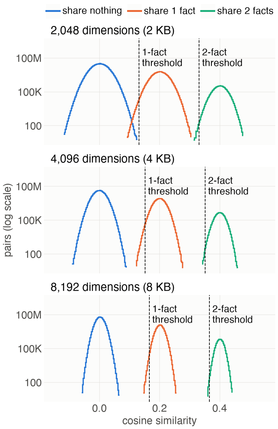
The measurements match the theory on every point it predicted. The peaks sit at 0, 0.2 and 0.4 at every dimension, so cosine similarity reliably tells us how many facts two records share. The curves also narrow as the dimension grows, meaning each pair’s cosine similarity strays less from the value its shared facts predict, which leaves more room between unrelated pairs and real matches.

At 2,048 dimensions, that room is just barely enough. The highest unrelated pairs reach 0.132 on average, equalling the threshold, so in this case, a false positive is rare but possible. Meanwhile, less than 0.06% of genuine one-fact matches fall below the threshold, so it keeps almost every real match, as designed.

From a practitioner’s perspective, this shows that the dimension decides how much margin a threshold has. At 2,048 dimensions, one-fact matching has almost no margin to spare, so a task that makes many comparisons will eventually hit a false positive, which E2 tests next.

E2: Does the number of comparisons decide the outcome?

E2 tests the second factor, the one the birthday paradox describes. Earlier, the theory predicted that with the records and the dimension held fixed, the chance of at least one false positive depends on which question the app asks. At 2,048 dimensions and 40,000 people, that chance is about 0.004% when checking whether anyone unrelated looks like Maya, and about 60% when checking whether any two unrelated people look alike.

The figure below shows how the chance of at least one false positive grows as we add people at 2,048 dimensions, with lines for the theory’s predictions and circles for our measurements.

Both lines share the same chance per comparison. They differ only in how many comparisons they make. Doubling the number of people doubles Maya’s comparisons but roughly quadruples the number of pairs. The red line for comparing any two people should therefore climb far faster, and that widening gap is the “birthday paradox” in our data.

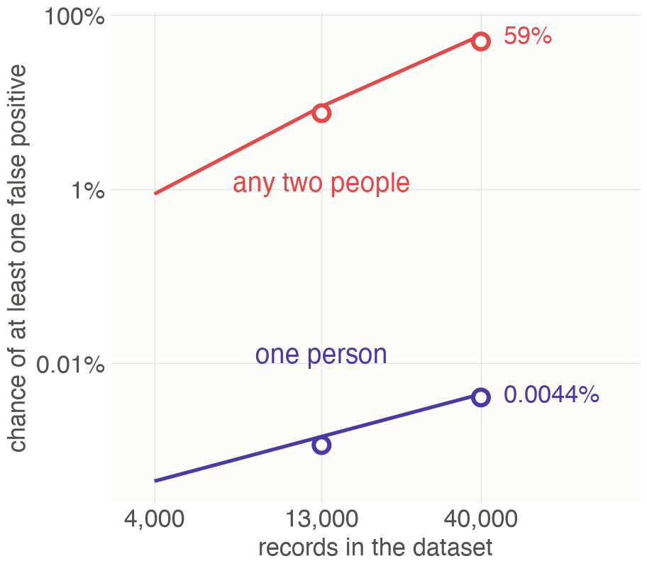
At 2,048 dimensions, we repeated the experiment 40 times, each time with fresh random hypervectors. For any two people, the measured chance is the share of these 40 runs with at least one false positive.

For one person, a single search almost never returns a false positive, so we treat each person’s comparisons as their own search, as if each were Maya, and measure the share of searches that return one. The chart below compares these measurements with the theory’s predictions:

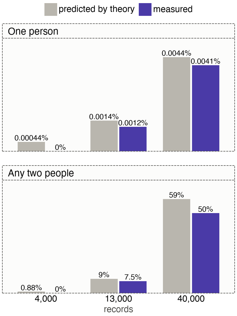
The measured bars sit close to the predictions in both panels. Counting comparisons accounts for the risk in a single search and across all pairs. Some variation is expected with rare events: the largest gap, 50% against 59%, is still consistent with the variation expected from 40 runs.

As predicted, no false positive appeared in any run at 4,096 or 8,192 dimensions, or when a match required two shared facts. In each case, the chance per comparison falls so low that even 800 million comparisons aren’t enough to produce an accidental match.

Estimated capacity at each dimension

With both factors confirmed, we can return to the opening question. Keeping the chance of any false positive at or below 1%, and solving $M\,p(T)$ for the number of records $N$, gives:

Dimensions	Storage per hypervector	A match means	One person’s search	Everyone with everyone
2,048	2 KB	1+ shared fact	about 9 million	about 4,200
2,048	2 KB	2+ shared facts	about $3 \times 10^{49}$	about $8 \times 10^{24}$
4,096	4 KB	1+ shared fact	about $10^{20}$	about 14 billion
8,192	8 KB	1+ shared fact	about $7 \times 10^{48}$	about $4 \times 10^{24}$

Each number is the largest dataset that keeps the chance of any false positive at or below 1%. In the first row, with 2,048 dimensions and a match meaning at least one shared fact, Maya’s search stays within that limit up to about 9 million people. Comparing everyone with everyone reaches the same limit at only about 4,200 people. The dimension and the encoding are identical in both columns, so the whole gap comes from the number of comparisons.

These are estimates from the validated theory, not measurements, and they assume independent, evenly spread properties. A practitioner can raise these numbers in three ways:

• Increase the dimension. Each comparison becomes less likely to produce a false positive.
• Reduce the number of comparisons. Searching for one record at a time makes far fewer comparisons than comparing every pair.
• Require more shared facts for a match. This is the most effective of the three: at 2,048 dimensions, it raises the capacity for comparing everyone with everyone from about 4,200 records to about $8 \times 10^{24}$.

Capacity is also highly sensitive to how the records are encoded. Before running these experiments, we estimated on paper that 2,048 dimensions could hold about 17.3 billion records when comparing everyone with everyone on two-fact matches, far fewer than the $8 \times 10^{24}$ in our table. The difference comes from one encoding choice: that estimate kept only the sign of each element in the bundle, which lowers the cosine similarity of a two-fact match from 0.4 to about 0.28. Small choices like this can move capacity by many orders of magnitude.

Conclusions

We set out to find how many records a 2,048-dimensional hyperspace can hold before unrelated records start to look alike. The theory gave us two factors to work with: the chance that a single comparison produces a false positive, set by the dimension, and the number of comparisons, set by the question the application asks. Our experiments on 40,000 records confirmed both, closely enough that the theory can be trusted to estimate capacity well beyond what we measured.

Whether a hyperspace is big enough doesn’t depend on its dimension alone. It also depends on how many comparisons the application makes, and on how much information two records must share to count as a match. Our findings indicate that a hyperspace’s capacity grows remarkably fast with the number of dimensions.

When everyone is compared with everyone else, 2,048 dimensions keep the chance of any false positive under 1% for only about 4,200 records. Doubling to 4,096 dimensions raises that to about 14 billion records, because each comparison becomes about ten trillion times less likely to mistake two unrelated records for a match.

In a future post, we’ll look at what happens when records come with missing properties. Stay tuned!

The experiment repository ↗ contains the report, methodology, source code, and reproduction steps.

Footnotes

1. Here, every property contributes an equal share to the cosine similarity. Other applications can weight each property differently, depending on what a match should capture, such as counting a shared employer for more than a shared region. ↩

2. If each of $D$ elements agrees with probability one half, the number of agreeing elements follows a binomial distribution, and the cosine similarity is the share of agreements minus the share of disagreements. The implementation evaluates the chance of reaching a threshold with SciPy’s binomial survival function ↗ . The model is exact for records whose elements are all $\pm1$. Our raw-sum records take values from $-5$ to $5$, but unrelated pairs still average 0 with a spread of $1/\sqrt D$, and the experiments show that the model predicts their false positives closely. ↩